SDS-2.2, Scalable Data Science
Archived YouTube video of this live unedited lab-lecture:
Power Plant ML Pipeline Application
This is an end-to-end example of using a number of different machine learning algorithms to solve a supervised regression problem.
Table of Contents
- Step 1: Business Understanding
- Step 2: Load Your Data
- Step 3: Explore Your Data
- Step 4: Visualize Your Data
- Step 5: Data Preparation
- Step 6: Data Modeling
- Step 7: Tuning and Evaluation
- Step 8: Deployment
We are trying to predict power output given a set of readings from various sensors in a gas-fired power generation plant. Power generation is a complex process, and understanding and predicting power output is an important element in managing a plant and its connection to the power grid.
More information about Peaker or Peaking Power Plants can be found on Wikipedia https://en.wikipedia.org/wiki/Peaking*power*plant
Given this business problem, we need to translate it to a Machine Learning task. The ML task is regression since the label (or target) we are trying to predict is numeric.
The example data is provided by UCI at UCI Machine Learning Repository Combined Cycle Power Plant Data Set
You can read the background on the UCI page, but in summary we have collected a number of readings from sensors at a Gas Fired Power Plant
(also called a Peaker Plant) and now we want to use those sensor readings to predict how much power the plant will generate.
More information about Machine Learning with Spark can be found in the Spark MLLib Programming Guide
Please note this example only works with Spark version 1.4 or higher
To Rerun Steps 1-4 done in the notebook at:
just run the following command as shown in the cell below:
%run "/scalable-data-science/sds-2-2/009_PowerPlantPipeline_01ETLEDA"
Note: If you already evaluated the
%run ...command above then:- first delete the cell by pressing on
xon the top-right corner of the cell and - revaluate the
runcommand above.
- first delete the cell by pressing on
"/scalable-data-science/sds-2-2/009_PowerPlantPipeline_01ETLEDA"
Now we will do the following Steps:
Step 5: Data Preparation,
Step 6: Modeling, and
Step 7: Tuning and Evaluation
We will do Step 8: Deployment later after we get introduced to SparkStreaming.
Step 5: Data Preparation
The next step is to prepare the data. Since all of this data is numeric and consistent, this is a simple task for us today.
We will need to convert the predictor features from columns to Feature Vectors using the org.apache.spark.ml.feature.VectorAssembler
The VectorAssembler will be the first step in building our ML pipeline.
//Let's quickly recall the schema and make sure our table is here now
table("power_plant_table").printSchema
root
 |-- AT: double (nullable = true)
 |-- V: double (nullable = true)
 |-- AP: double (nullable = true)
 |-- RH: double (nullable = true)
 |-- PE: double (nullable = true)
powerPlantDF // make sure we have the DataFrame too
res23: org.apache.spark.sql.DataFrame = [AT: double, V: double ... 3 more fields]
import org.apache.spark.ml.feature.VectorAssembler

// make a DataFrame called dataset from the table
val dataset = sqlContext.table("power_plant_table")

val vectorizer =  new VectorAssembler()
                      .setInputCols(Array("AT", "V", "AP", "RH"))
                      .setOutputCol("features")
import org.apache.spark.ml.feature.VectorAssembler
dataset: org.apache.spark.sql.DataFrame = [AT: double, V: double ... 3 more fields]
vectorizer: org.apache.spark.ml.feature.VectorAssembler = vecAssembler_bca323dc00ef
Step 6: Data Modeling
Now let's model our data to predict what the power output will be given a set of sensor readings
Our first model will be based on simple linear regression since we saw some linear patterns in our data based on the scatter plots during the exploration stage.
Linear Regression Model
- Linear Regression is one of the most useful work-horses of statistical learning
- See Chapter 7 of Kevin Murphy's Machine Learning froma Probabilistic Perspective for a good mathematical and algorithmic introduction.
- You should have already seen Ameet's treatment of the topic from earlier notebook.
Let's open http://spark.apache.org/docs/latest/mllib-linear-methods.html#regression for some details.
// First let's hold out 20% of our data for testing and leave 80% for training
var Array(split20, split80) = dataset.randomSplit(Array(0.20, 0.80), 1800009193L)
split20: org.apache.spark.sql.Dataset[org.apache.spark.sql.Row] = [AT: double, V: double ... 3 more fields]
split80: org.apache.spark.sql.Dataset[org.apache.spark.sql.Row] = [AT: double, V: double ... 3 more fields]
// Let's cache these datasets for performance
val testSet = split20.cache()
val trainingSet = split80.cache()
testSet: org.apache.spark.sql.Dataset[org.apache.spark.sql.Row] = [AT: double, V: double ... 3 more fields]
trainingSet: org.apache.spark.sql.Dataset[org.apache.spark.sql.Row] = [AT: double, V: double ... 3 more fields]
testSet.count() // action to actually cache
res27: Long = 1966
trainingSet.count() // action to actually cache
res28: Long = 7602
Let's take a few elements of the three DataFrames.
dataset.take(3)
res24: Array[org.apache.spark.sql.Row] = Array([14.96,41.76,1024.07,73.17,463.26], [25.18,62.96,1020.04,59.08,444.37], [5.11,39.4,1012.16,92.14,488.56])
testSet.take(3)
res25: Array[org.apache.spark.sql.Row] = Array([1.81,39.42,1026.92,76.97,490.55], [3.2,41.31,997.67,98.84,489.86], [3.38,41.31,998.79,97.76,489.11])
trainingSet.take(3)
res26: Array[org.apache.spark.sql.Row] = Array([2.34,39.42,1028.47,69.68,490.34], [2.58,39.42,1028.68,69.03,488.69], [2.64,39.64,1011.02,85.24,481.29])
// ***** LINEAR REGRESSION MODEL ****

import org.apache.spark.ml.regression.LinearRegression
import org.apache.spark.ml.regression.LinearRegressionModel
import org.apache.spark.ml.Pipeline

// Let's initialize our linear regression learner
val lr = new LinearRegression()
import org.apache.spark.ml.regression.LinearRegression
import org.apache.spark.ml.regression.LinearRegressionModel
import org.apache.spark.ml.Pipeline
lr: org.apache.spark.ml.regression.LinearRegression = linReg_161e726c1f38
// We use explain params to dump the parameters we can use
lr.explainParams()
res29: String =
aggregationDepth: suggested depth for treeAggregate (>= 2) (default: 2)
elasticNetParam: the ElasticNet mixing parameter, in range [0, 1]. For alpha = 0, the penalty is an L2 penalty. For alpha = 1, it is an L1 penalty (default: 0.0)
featuresCol: features column name (default: features)
fitIntercept: whether to fit an intercept term (default: true)
labelCol: label column name (default: label)
maxIter: maximum number of iterations (>= 0) (default: 100)
predictionCol: prediction column name (default: prediction)
regParam: regularization parameter (>= 0) (default: 0.0)
solver: the solver algorithm for optimization. If this is not set or empty, default value is 'auto' (default: auto)
standardization: whether to standardize the training features before fitting the model (default: true)
tol: the convergence tolerance for iterative algorithms (>= 0) (default: 1.0E-6)
weightCol: weight column name. If this is not set or empty, we treat all instance weights as 1.0 (undefined)
The cell below is based on the Spark ML pipeline API. More information can be found in the Spark ML Programming Guide at https://spark.apache.org/docs/latest/ml-guide.html
// Now we set the parameters for the method
lr.setPredictionCol("Predicted_PE")
  .setLabelCol("PE")
  .setMaxIter(100)
  .setRegParam(0.1)
// We will use the new spark.ml pipeline API. If you have worked with scikit-learn this will be very familiar.
val lrPipeline = new Pipeline()
lrPipeline.setStages(Array(vectorizer, lr))
// Let's first train on the entire dataset to see what we get
val lrModel = lrPipeline.fit(trainingSet)
lrPipeline: org.apache.spark.ml.Pipeline = pipeline_8b0213f4b86e
lrModel: org.apache.spark.ml.PipelineModel = pipeline_8b0213f4b86e
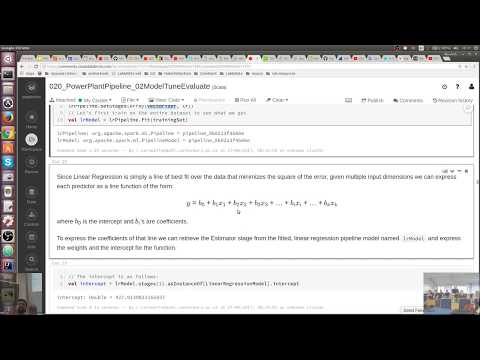
Since Linear Regression is simply a line of best fit over the data that minimizes the square of the error, given multiple input dimensions we can express each predictor as a line function of the form:
where is the intercept and 's are coefficients.
To express the coefficients of that line we can retrieve the Estimator stage from the fitted, linear-regression pipeline model named lrModel and express the weights and the intercept for the function.
// The intercept is as follows:
val intercept = lrModel.stages(1).asInstanceOf[LinearRegressionModel].intercept
intercept: Double = 427.9139822165837
// The coefficents (i.e. weights) are as follows:

val weights = lrModel.stages(1).asInstanceOf[LinearRegressionModel].coefficients.toArray
weights: Array[Double] = Array(-1.9083064919040942, -0.25381293007161654, 0.08739350304730673, -0.1474651301033126)
The model has been fit and the intercept and coefficients displayed above.
Now, let us do some work to make a string of the model that is easy to understand for an applied data scientist or data analyst.
val featuresNoLabel = dataset.columns.filter(col => col != "PE")
featuresNoLabel: Array[String] = Array(AT, V, AP, RH)
val coefficentFeaturePairs = sc.parallelize(weights).zip(sc.parallelize(featuresNoLabel))
coefficentFeaturePairs: org.apache.spark.rdd.RDD[(Double, String)] = ZippedPartitionsRDD2[35297] at zip at <console>:42
coefficentFeaturePairs.collect() // this just pairs each coefficient with the name of its corresponding feature
res30: Array[(Double, String)] = Array((-1.9083064919040942,AT), (-0.25381293007161654,V), (0.08739350304730673,AP), (-0.1474651301033126,RH))
// Now let's sort the coefficients from the largest to the smallest

var equation = s"y = $intercept "
//var variables = Array
coefficentFeaturePairs.sortByKey().collect().foreach({
  case (weight, feature) =>
  {
        val symbol = if (weight > 0) "+" else "-"
        val absWeight = Math.abs(weight)
        equation += (s" $symbol (${absWeight} * ${feature})")
  }
}
)
equation: String = y = 427.9139822165837 - (1.9083064919040942 * AT) - (0.25381293007161654 * V) - (0.1474651301033126 * RH) + (0.08739350304730673 * AP)
// Finally here is our equation
println("Linear Regression Equation: " + equation)
Linear Regression Equation: y = 427.9139822165837 - (1.9083064919040942 * AT) - (0.25381293007161654 * V) - (0.1474651301033126 * RH) + (0.08739350304730673 * AP)
Based on examining the fitted Linear Regression Equation above:
- There is a strong negative correlation between Atmospheric Temperature (AT) and Power Output due to the coefficient being greater than -1.91.
- But our other dimenensions seem to have little to no correlation with Power Output.
Do you remember Step 2: Explore Your Data? When we visualized each predictor against Power Output using a Scatter Plot, only the temperature variable seemed to have a linear correlation with Power Output so our final equation seems logical.
Now let's see what our predictions look like given this model.
val predictionsAndLabels = lrModel.transform(testSet)

display(predictionsAndLabels.select("AT", "V", "AP", "RH", "PE", "Predicted_PE"))
| AT | V | AP | RH | PE | Predicted_PE |
|---|---|---|---|---|---|
| 1.81 | 39.42 | 1026.92 | 76.97 | 490.55 | 492.8503868481024 |
| 3.2 | 41.31 | 997.67 | 98.84 | 489.86 | 483.9368120270272 |
| 3.38 | 41.31 | 998.79 | 97.76 | 489.11 | 483.850459922409 |
| 3.4 | 39.64 | 1011.1 | 83.43 | 459.86 | 487.4251507226833 |
| 3.51 | 35.47 | 1017.53 | 86.56 | 489.07 | 488.37401129434335 |
| 3.63 | 38.44 | 1016.16 | 87.38 | 487.87 | 487.1505396071426 |
| 3.91 | 35.47 | 1016.92 | 86.03 | 488.67 | 487.6355351796776 |
| 3.94 | 39.9 | 1008.06 | 97.49 | 488.81 | 483.9896378767201 |
| 4.0 | 39.9 | 1009.64 | 97.16 | 490.79 | 484.0618847149547 |
| 4.15 | 39.9 | 1007.62 | 95.69 | 489.8 | 483.8158776062654 |
| 4.15 | 39.9 | 1008.84 | 96.68 | 491.22 | 483.77650720118083 |
| 4.23 | 38.44 | 1016.46 | 76.64 | 489.0 | 487.61554926022393 |
| 4.24 | 39.9 | 1009.28 | 96.74 | 491.25 | 483.6343648504441 |
| 4.43 | 38.91 | 1019.04 | 88.17 | 491.9 | 485.6397981724803 |
| 4.44 | 38.44 | 1016.14 | 75.35 | 486.53 | 487.37706899378225 |
| 4.61 | 40.27 | 1012.32 | 77.28 | 492.85 | 485.96972834538735 |
| 4.65 | 35.19 | 1018.23 | 94.78 | 489.36 | 485.11862159667663 |
| 4.69 | 39.42 | 1024.58 | 79.35 | 486.34 | 486.79899634464203 |
| 4.73 | 41.31 | 999.77 | 93.44 | 486.6 | 481.99694115337115 |
| 4.77 | 39.33 | 1011.32 | 68.98 | 494.91 | 487.0395505377602 |
| 4.78 | 42.85 | 1013.39 | 93.36 | 481.47 | 482.7127506383782 |
| 4.83 | 38.44 | 1015.35 | 72.94 | 485.32 | 486.9191795580812 |
| 4.86 | 39.4 | 1012.73 | 91.39 | 488.63 | 483.6685673220653 |
| 4.89 | 45.87 | 1007.58 | 99.35 | 482.69 | 480.3452494934288 |
| 4.95 | 42.07 | 1004.87 | 80.88 | 485.67 | 483.6820847979367 |
| 4.96 | 39.4 | 1003.58 | 92.22 | 486.09 | 482.5556900620063 |
| 4.96 | 40.07 | 1011.8 | 67.38 | 494.75 | 486.76704382567345 |
| 5.07 | 40.07 | 1019.32 | 66.17 | 494.87 | 487.39276206190476 |
| 5.19 | 40.78 | 1025.24 | 95.07 | 482.46 | 483.2391853805797 |
| 5.24 | 38.68 | 1018.03 | 78.65 | 486.67 | 485.46804748846023 |
Truncated to 30 rows
Now that we have real predictions we can use an evaluation metric such as Root Mean Squared Error to validate our regression model. The lower the Root Mean Squared Error, the better our model.
//Now let's compute some evaluation metrics against our test dataset

import org.apache.spark.mllib.evaluation.RegressionMetrics

val metrics = new RegressionMetrics(predictionsAndLabels.select("Predicted_PE", "PE").rdd.map(r => (r(0).asInstanceOf[Double], r(1).asInstanceOf[Double])))
import org.apache.spark.mllib.evaluation.RegressionMetrics
metrics: org.apache.spark.mllib.evaluation.RegressionMetrics = org.apache.spark.mllib.evaluation.RegressionMetrics@32433b70
val rmse = metrics.rootMeanSquaredError
rmse: Double = 4.609375859170583
val explainedVariance = metrics.explainedVariance
explainedVariance: Double = 274.54186073318266
val r2 = metrics.r2
r2: Double = 0.9308377700269259
println (f"Root Mean Squared Error: $rmse")
println (f"Explained Variance: $explainedVariance")
println (f"R2: $r2")
Root Mean Squared Error: 4.609375859170583
Explained Variance: 274.54186073318266
R2: 0.9308377700269259
Generally a good model will have 68% of predictions within 1 RMSE and 95% within 2 RMSE of the actual value. Let's calculate and see if our RMSE meets this criteria.
display(predictionsAndLabels) // recall the DataFrame predictionsAndLabels
// First we calculate the residual error and divide it by the RMSE from predictionsAndLabels DataFrame and make another DataFrame that is registered as a temporary table Power_Plant_RMSE_Evaluation
predictionsAndLabels.selectExpr("PE", "Predicted_PE", "PE - Predicted_PE AS Residual_Error", s""" (PE - Predicted_PE) / $rmse AS Within_RSME""").createOrReplaceTempView("Power_Plant_RMSE_Evaluation")
SELECT * from Power_Plant_RMSE_Evaluation
| PE | Predicted_PE | Residual_Error | Within_RSME |
|---|---|---|---|
| 490.55 | 492.8503868481024 | -2.3003868481023915 | -0.49906688419119855 |
| 489.86 | 483.9368120270272 | 5.923187972972812 | 1.2850303715606821 |
| 489.11 | 483.850459922409 | 5.259540077590998 | 1.1410525499080058 |
| 459.86 | 487.4251507226833 | -27.565150722683313 | -5.980234974295072 |
| 489.07 | 488.37401129434335 | 0.6959887056566458 | 0.15099413172652035 |
| 487.87 | 487.1505396071426 | 0.7194603928573997 | 0.1560862934243033 |
| 488.67 | 487.6355351796776 | 1.0344648203223983 | 0.22442622427161782 |
| 488.81 | 483.9896378767201 | 4.820362123279892 | 1.045773282664624 |
| 490.79 | 484.0618847149547 | 6.728115285045305 | 1.4596586372229519 |
| 489.8 | 483.8158776062654 | 5.984122393734594 | 1.2982500400415133 |
| 491.22 | 483.77650720118083 | 7.443492798819193 | 1.6148591536552597 |
| 489.0 | 487.61554926022393 | 1.3844507397760708 | 0.30035535874594327 |
| 491.25 | 483.6343648504441 | 7.615635149555885 | 1.6522052838030554 |
| 491.9 | 485.6397981724803 | 6.260201827519666 | 1.3581452280713195 |
| 486.53 | 487.37706899378225 | -0.8470689937822726 | -0.1837708660917696 |
| 492.85 | 485.96972834538735 | 6.88027165461267 | 1.4926688265015375 |
| 489.36 | 485.11862159667663 | 4.241378403323381 | 0.9201632786974722 |
| 486.34 | 486.79899634464203 | -0.45899634464205974 | -9.957884942900971e-2 |
| 486.6 | 481.99694115337115 | 4.603058846628869 | 0.9986295297379263 |
| 494.91 | 487.0395505377602 | 7.870449462239833 | 1.707487022691192 |
| 481.47 | 482.7127506383782 | -1.2427506383781974 | -0.26961364756264844 |
| 485.32 | 486.9191795580812 | -1.5991795580812322 | -0.346940585220358 |
| 488.63 | 483.6685673220653 | 4.961432677934681 | 1.076378414240979 |
| 482.69 | 480.3452494934288 | 2.344750506571188 | 0.5086915405056825 |
| 485.67 | 483.6820847979367 | 1.9879152020633342 | 0.4312764380253951 |
| 486.09 | 482.5556900620063 | 3.534309937993669 | 0.766765402947556 |
| 494.75 | 486.76704382567345 | 7.982956174326546 | 1.7318952539841284 |
| 494.87 | 487.39276206190476 | 7.477237938095243 | 1.6221801316590196 |
| 482.46 | 483.2391853805797 | -0.7791853805797473 | -0.16904357648108023 |
| 486.67 | 485.46804748846023 | 1.2019525115397869 | 0.26076253016955486 |
Truncated to 30 rows
-- Now we can display the RMSE as a Histogram. Clearly this shows that the RMSE is centered around 0 with the vast majority of the error within 2 RMSEs.
SELECT Within_RSME  from Power_Plant_RMSE_Evaluation
| Within_RSME |
|---|
| -0.49906688419119855 |
| 1.2850303715606821 |
| 1.1410525499080058 |
| -5.980234974295072 |
| 0.15099413172652035 |
| 0.1560862934243033 |
| 0.22442622427161782 |
| 1.045773282664624 |
| 1.4596586372229519 |
| 1.2982500400415133 |
| 1.6148591536552597 |
| 0.30035535874594327 |
| 1.6522052838030554 |
| 1.3581452280713195 |
| -0.1837708660917696 |
| 1.4926688265015375 |
| 0.9201632786974722 |
| -9.957884942900971e-2 |
| 0.9986295297379263 |
| 1.707487022691192 |
| -0.26961364756264844 |
| -0.346940585220358 |
| 1.076378414240979 |
| 0.5086915405056825 |
| 0.4312764380253951 |
| 0.766765402947556 |
| 1.7318952539841284 |
| 1.6221801316590196 |
| -0.16904357648108023 |
| 0.26076253016955486 |
Truncated to 30 rows
We can see this definitively if we count the number of predictions within + or - 1.0 and + or - 2.0 and display this as a pie chart:
SELECT case when Within_RSME <= 1.0 and Within_RSME >= -1.0 then 1  when  Within_RSME <= 2.0 and Within_RSME >= -2.0 then 2 else 3 end RSME_Multiple, COUNT(*) count  from Power_Plant_RMSE_Evaluation
group by case when Within_RSME <= 1.0 and Within_RSME >= -1.0 then 1  when  Within_RSME <= 2.0 and Within_RSME >= -2.0 then 2 else 3 end
| RSME_Multiple | count |
|---|---|
| 1.0 | 1312.0 |
| 3.0 | 55.0 |
| 2.0 | 599.0 |
So we have about 70% of our training data within 1 RMSE and about 97% (70% + 27%) within 2 RMSE. So the model is pretty decent. Let's see if we can tune the model to improve it further.
NOTE: these numbers will vary across runs due to the seed in random sampling of training and test set, number of iterations, and other stopping rules in optimization, for example.
Step 7: Tuning and Evaluation
Now that we have a model with all of the data let's try to make a better model by tuning over several parameters.
import org.apache.spark.ml.tuning.{ParamGridBuilder, CrossValidator}
import org.apache.spark.ml.evaluation._
import org.apache.spark.ml.tuning.{ParamGridBuilder, CrossValidator}
import org.apache.spark.ml.evaluation._
First let's use a cross validator to split the data into training and validation subsets. See http://spark.apache.org/docs/latest/ml-tuning.html.
//Let's set up our evaluator class to judge the model based on the best root mean squared error
val regEval = new RegressionEvaluator()
regEval.setLabelCol("PE")
  .setPredictionCol("Predicted_PE")
  .setMetricName("rmse")
regEval: org.apache.spark.ml.evaluation.RegressionEvaluator = regEval_c6d2feda2ee0
res37: regEval.type = regEval_c6d2feda2ee0
We now treat the lrPipeline as an Estimator, wrapping it in a CrossValidator instance.
This will allow us to jointly choose parameters for all Pipeline stages.
A CrossValidator requires an Estimator, an Evaluator (which we set next).
//Let's create our crossvalidator with 3 fold cross validation
val crossval = new CrossValidator()
crossval.setEstimator(lrPipeline)
crossval.setNumFolds(3)
crossval.setEvaluator(regEval)
crossval: org.apache.spark.ml.tuning.CrossValidator = cv_c77b278496fa
res38: crossval.type = cv_c77b278496fa
A CrossValidator also requires a set of EstimatorParamMaps which we set next.
For this we need a regularization parameter (more generally a hyper-parameter that is model-specific).
Now, let's tune over our regularization parameter from 0.01 to 0.10.
val regParam = ((1 to 10) toArray).map(x => (x /100.0))
warning: there was one feature warning; re-run with -feature for details
regParam: Array[Double] = Array(0.01, 0.02, 0.03, 0.04, 0.05, 0.06, 0.07, 0.08, 0.09, 0.1)
Check out the scala docs for syntactic details on org.apache.spark.ml.tuning.ParamGridBuilder.
val paramGrid = new ParamGridBuilder()
                    .addGrid(lr.regParam, regParam)
                    .build()
crossval.setEstimatorParamMaps(paramGrid)
paramGrid: Array[org.apache.spark.ml.param.ParamMap] =
Array({
    linReg_161e726c1f38-regParam: 0.01
}, {
    linReg_161e726c1f38-regParam: 0.02
}, {
    linReg_161e726c1f38-regParam: 0.03
}, {
    linReg_161e726c1f38-regParam: 0.04
}, {
    linReg_161e726c1f38-regParam: 0.05
}, {
    linReg_161e726c1f38-regParam: 0.06
}, {
    linReg_161e726c1f38-regParam: 0.07
}, {
    linReg_161e726c1f38-regParam: 0.08
}, {
    linReg_161e726c1f38-regParam: 0.09
}, {
    linReg_161e726c1f38-regParam: 0.1
})
res39: crossval.type = cv_c77b278496fa
//Now let's create our model
val cvModel = crossval.fit(trainingSet)
cvModel: org.apache.spark.ml.tuning.CrossValidatorModel = cv_c77b278496fa
In addition to CrossValidator Spark also offers TrainValidationSplit for hyper-parameter tuning. TrainValidationSplit only evaluates each combination of parameters once as opposed to k times in case of CrossValidator. It is therefore less expensive, but will not produce as reliable results when the training dataset is not sufficiently large.
Now that we have tuned let's see what we got for tuning parameters and what our RMSE was versus our intial model
val predictionsAndLabels = cvModel.transform(testSet)
val metrics = new RegressionMetrics(predictionsAndLabels.select("Predicted_PE", "PE").rdd.map(r => (r(0).asInstanceOf[Double], r(1).asInstanceOf[Double])))

val rmse = metrics.rootMeanSquaredError
val explainedVariance = metrics.explainedVariance
val r2 = metrics.r2
predictionsAndLabels: org.apache.spark.sql.DataFrame = [AT: double, V: double ... 5 more fields]
metrics: org.apache.spark.mllib.evaluation.RegressionMetrics = org.apache.spark.mllib.evaluation.RegressionMetrics@77606693
rmse: Double = 4.599964072968395
explainedVariance: Double = 277.2272873387723
r2: Double = 0.9311199234339246
println (f"Root Mean Squared Error: $rmse")
println (f"Explained Variance: $explainedVariance")
println (f"R2: $r2")
Root Mean Squared Error: 4.599964072968395
Explained Variance: 277.2272873387723
R2: 0.9311199234339246
Let us explore other models to see if we can predict the power output better
There are several families of models in Spark's scalable machine learning library:
So our initial untuned and tuned linear regression models are statistically identical.
Given that the only linearly correlated variable is Temperature, it makes sense try another machine learning method such a Decision Tree to handle non-linear data and see if we can improve our model
A Decision Tree creates a model based on splitting variables using a tree structure. We will first start with a single decision tree model.
Reference Decision Trees: https://en.wikipedia.org/wiki/Decision*tree*learning
//Let's build a decision tree pipeline
import org.apache.spark.ml.regression.DecisionTreeRegressor

// we are using a Decision Tree Regressor as opposed to a classifier we used for the hand-written digit classification problem
val dt = new DecisionTreeRegressor()
dt.setLabelCol("PE")
dt.setPredictionCol("Predicted_PE")
dt.setFeaturesCol("features")
dt.setMaxBins(100)

val dtPipeline = new Pipeline()
dtPipeline.setStages(Array(vectorizer, dt))
import org.apache.spark.ml.regression.DecisionTreeRegressor
dt: org.apache.spark.ml.regression.DecisionTreeRegressor = dtr_532b2d8e3739
dtPipeline: org.apache.spark.ml.Pipeline = pipeline_604afd9d7ee3
res41: dtPipeline.type = pipeline_604afd9d7ee3
//Let's just resuse our CrossValidator
crossval.setEstimator(dtPipeline)
res42: crossval.type = cv_c77b278496fa
val paramGrid = new ParamGridBuilder()
                     .addGrid(dt.maxDepth, Array(2, 3))
                     .build()
paramGrid: Array[org.apache.spark.ml.param.ParamMap] =
Array({
    dtr_532b2d8e3739-maxDepth: 2
}, {
    dtr_532b2d8e3739-maxDepth: 3
})
crossval.setEstimatorParamMaps(paramGrid)
res43: crossval.type = cv_c77b278496fa
val dtModel = crossval.fit(trainingSet) // fit decitionTree with cv
dtModel: org.apache.spark.ml.tuning.CrossValidatorModel = cv_c77b278496fa
import org.apache.spark.ml.regression.DecisionTreeRegressionModel
import org.apache.spark.ml.PipelineModel
dtModel.bestModel.asInstanceOf[PipelineModel].stages.last.asInstanceOf[DecisionTreeRegressionModel].toDebugString
import org.apache.spark.ml.regression.DecisionTreeRegressionModel
import org.apache.spark.ml.PipelineModel
res45: String =
"DecisionTreeRegressionModel (uid=dtr_532b2d8e3739) of depth 3 with 15 nodes
  If (feature 0 <= 17.84)
   If (feature 0 <= 11.95)
    If (feature 0 <= 8.75)
     Predict: 483.5412151067323
    Else (feature 0 > 8.75)
     Predict: 475.6305502392345
   Else (feature 0 > 11.95)
    If (feature 0 <= 15.33)
     Predict: 467.63141917293234
    Else (feature 0 > 15.33)
     Predict: 460.74754125412574
  Else (feature 0 > 17.84)
   If (feature 0 <= 23.02)
    If (feature 1 <= 47.83)
     Predict: 457.1077966101695
    Else (feature 1 > 47.83)
     Predict: 448.74750213858016
   Else (feature 0 > 23.02)
    If (feature 1 <= 66.25)
     Predict: 442.88544855967086
    Else (feature 1 > 66.25)
     Predict: 434.7293710691822
"
The line above will pull the Decision Tree model from the Pipeline and display it as an if-then-else string.
Next let's visualize it as a decision tree for regression.
display(dtModel.bestModel.asInstanceOf[PipelineModel].stages.last.asInstanceOf[DecisionTreeRegressionModel])
| treeNode |
|---|
| {"index":7,"featureType":"continuous","prediction":null,"threshold":17.84,"categories":null,"feature":0,"overflow":false} |
| {"index":3,"featureType":"continuous","prediction":null,"threshold":11.95,"categories":null,"feature":0,"overflow":false} |
| {"index":1,"featureType":"continuous","prediction":null,"threshold":8.75,"categories":null,"feature":0,"overflow":false} |
| {"index":0,"featureType":null,"prediction":483.5412151067323,"threshold":null,"categories":null,"feature":null,"overflow":false} |
| {"index":2,"featureType":null,"prediction":475.6305502392345,"threshold":null,"categories":null,"feature":null,"overflow":false} |
| {"index":5,"featureType":"continuous","prediction":null,"threshold":15.33,"categories":null,"feature":0,"overflow":false} |
| {"index":4,"featureType":null,"prediction":467.63141917293234,"threshold":null,"categories":null,"feature":null,"overflow":false} |
| {"index":6,"featureType":null,"prediction":460.74754125412574,"threshold":null,"categories":null,"feature":null,"overflow":false} |
| {"index":11,"featureType":"continuous","prediction":null,"threshold":23.02,"categories":null,"feature":0,"overflow":false} |
| {"index":9,"featureType":"continuous","prediction":null,"threshold":47.83,"categories":null,"feature":1,"overflow":false} |
| {"index":8,"featureType":null,"prediction":457.1077966101695,"threshold":null,"categories":null,"feature":null,"overflow":false} |
| {"index":10,"featureType":null,"prediction":448.74750213858016,"threshold":null,"categories":null,"feature":null,"overflow":false} |
| {"index":13,"featureType":"continuous","prediction":null,"threshold":66.25,"categories":null,"feature":1,"overflow":false} |
| {"index":12,"featureType":null,"prediction":442.88544855967086,"threshold":null,"categories":null,"feature":null,"overflow":false} |
| {"index":14,"featureType":null,"prediction":434.7293710691822,"threshold":null,"categories":null,"feature":null,"overflow":false} |
Now let's see how our DecisionTree model compares to our LinearRegression model
val predictionsAndLabels = dtModel.bestModel.transform(testSet)
val metrics = new RegressionMetrics(predictionsAndLabels.select("Predicted_PE", "PE").map(r => (r(0).asInstanceOf[Double], r(1).asInstanceOf[Double])).rdd)

val rmse = metrics.rootMeanSquaredError
val explainedVariance = metrics.explainedVariance
val r2 = metrics.r2

println (f"Root Mean Squared Error: $rmse")
println (f"Explained Variance: $explainedVariance")
println (f"R2: $r2")
Root Mean Squared Error: 5.221342219456633
Explained Variance: 269.66550072645475
R2: 0.9112539444165726
predictionsAndLabels: org.apache.spark.sql.DataFrame = [AT: double, V: double ... 5 more fields]
metrics: org.apache.spark.mllib.evaluation.RegressionMetrics = org.apache.spark.mllib.evaluation.RegressionMetrics@2e492425
rmse: Double = 5.221342219456633
explainedVariance: Double = 269.66550072645475
r2: Double = 0.9112539444165726
So our DecisionTree was slightly worse than our LinearRegression model (LR: 4.6 vs DT: 5.2). Maybe we can try an Ensemble method such as Gradient-Boosted Decision Trees to see if we can strengthen our model by using an ensemble of weaker trees with weighting to reduce the error in our model.
Note since this is a complex model, the cell below can take about 16 minutes* or so to run on a small cluster with a couple nodes with about 6GB RAM, go out and grab a coffee and come back :-).*
This GBTRegressor code will be way faster on a larger cluster of course.
A visual explanation of gradient boosted trees:
Let's see what a boosting algorithm, a type of ensemble method, is all about in more detail.
import org.apache.spark.ml.regression.GBTRegressor

val gbt = new GBTRegressor()
gbt.setLabelCol("PE")
gbt.setPredictionCol("Predicted_PE")
gbt.setFeaturesCol("features")
gbt.setSeed(100088121L)
gbt.setMaxBins(100)
gbt.setMaxIter(120)

val gbtPipeline = new Pipeline()
gbtPipeline.setStages(Array(vectorizer, gbt))
//Let's just resuse our CrossValidator

crossval.setEstimator(gbtPipeline)

val paramGrid = new ParamGridBuilder()
  .addGrid(gbt.maxDepth, Array(2, 3))
  .build()
crossval.setEstimatorParamMaps(paramGrid)

//gbt.explainParams
val gbtModel = crossval.fit(trainingSet)
import org.apache.spark.ml.regression.GBTRegressionModel

val predictionsAndLabels = gbtModel.bestModel.transform(testSet)
val metrics = new RegressionMetrics(predictionsAndLabels.select("Predicted_PE", "PE").map(r => (r(0).asInstanceOf[Double], r(1).asInstanceOf[Double])).rdd)

val rmse = metrics.rootMeanSquaredError
val explainedVariance = metrics.explainedVariance
val r2 = metrics.r2


println (f"Root Mean Squared Error: $rmse")
println (f"Explained Variance: $explainedVariance")
println (f"R2: $r2")
We can use the toDebugString method to dump out what our trees and weighting look like:
gbtModel.bestModel.asInstanceOf[PipelineModel].stages.last.asInstanceOf[GBTRegressionModel].toDebugString
Conclusion
Wow! So our best model is in fact our Gradient Boosted Decision tree model which uses an ensemble of 120 Trees with a depth of 3 to construct a better model than the single decision tree.
Step 8: Deployment will be done later
Now that we have a predictive model it is time to deploy the model into an operational environment.
In our example, let's say we have a series of sensors attached to the power plant and a monitoring station.
The monitoring station will need close to real-time information about how much power that their station will generate so they can relay that to the utility.
For this we need to create a Spark Streaming utility that we can use for this purpose. For this you need to be introduced to basic concepts in Spark Streaming first. See http://spark.apache.org/docs/latest/streaming-programming-guide.html if you can't wait!
After deployment you will be able to use the best predictions from gradient boosed regression trees to feed a real-time dashboard or feed the utility with information on how much power the peaker plant will deliver give current conditions.
Datasource References:
- Pinar Tüfekci, Prediction of full load electrical power output of a base load operated combined cycle power plant using machine learning methods, International Journal of Electrical Power & Energy Systems, Volume 60, September 2014, Pages 126-140, ISSN 0142-0615, Web Link
- Heysem Kaya, Pinar Tüfekci , Sadik Fikret Gürgen: Local and Global Learning Methods for Predicting Power of a Combined Gas & Steam Turbine, Proceedings of the International Conference on Emerging Trends in Computer and Electronics Engineering ICETCEE 2012, pp. 13-18 (Mar. 2012, Dubai) Web Link