SDS-2.2, Scalable Data Science
Archived YouTube video of this live unedited lab-lecture:


What is Geospatial Analytics?
(watch now 3 minutes and 23 seconds: 111-314 seconds):
Some Concrete Examples of Scalable Geospatial Analytics
Let us check out cross-domain data fusion in MSR's Urban Computing Group
- lots of interesting papers to read at http://research.microsoft.com/en-us/projects/urbancomputing/.
Several sciences are naturally geospatial
- forestry,
- geography,
- geology,
- seismology,
- etc. etc.
See for example the global EQ datastreams from US geological Service below.
For a global data source, see US geological Service's Earthquake hazards Program "http://earthquake.usgs.gov/data/.
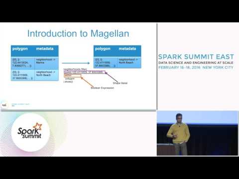
Introduction to Magellan for Scalable Geospatial Analytics
This is a minor augmentation of Ram Harsha's Magellan code blogged here:
First you need to attach the following library:
- the magellan library (maven coordinates
harsha2010:magellan:1.0.5-s_2.11)
Do we need one more geospatial analytics library?
From Ram's slide 4 of this Spark Summit East 2016 talk at slideshare:
- Spatial Analytics at scale is challenging
- Simplicity + Scalability = Hard
- Ancient Data Formats
- metadata, indexing not handled well, inefficient storage
- Geospatial Analytics is not simply Business Intelligence anymore
- Statistical + Machine Learning being leveraged in geospatial
- Now is the time to do it!
- Explosion of mobile data
- Finer granularity of data collection for geometries
- Analytics stretching the limits of traditional approaches
- Spark SQL + Catalyst + Tungsten makes extensible SQL engines easier than ever before!
Nuts and Bolts of Magellan
Let us go and grab this databricks notebook:
and look at the magellan README in github:
HOMEWORK: Watch the magellan presentation by Ram Harsha (Hortonworks) in Spark Summit East 2016.
Other resources for magellan:
- Ram's blog in HortonWorks and the ZeppelinHub view of the demo code in video above
- Magellan as Spark project and Magellan github source
- shape files developed by Environmental Systems Research Institute (ESRI). See ESRI's what is a geospatial shape file?
- magellan builds on http://esri.github.io/ a leading opensource geospatial library
Let's get our hands dirty with basics in magellan.
Data Structures
- Points
- Polygons
- lines
- Polylines
Predicates
- within
- intersects
// create a points DataFrame
val points = sc.parallelize(Seq((-1.0, -1.0), (-1.0, 1.0), (1.0, -1.0))).toDF("x", "y")
points: org.apache.spark.sql.DataFrame = [x: double, y: double]
// transform (lat,lon) into Point using custom user-defined function
import magellan.Point
import org.apache.spark.sql.functions.udf
val toPointUDF = udf{(x:Double,y:Double) => Point(x,y) }
import magellan.Point
import org.apache.spark.sql.functions.udf
toPointUDF: org.apache.spark.sql.expressions.UserDefinedFunction = UserDefinedFunction(<function2>,org.apache.spark.sql.types.PointUDT@105fcd11,Some(List(DoubleType, DoubleType)))
// let's show the results of the DF with a new column called point
points.withColumn("point", toPointUDF('x, 'y)).show()
+----+----+-----------------+
|   x|   y|            point|
+----+----+-----------------+
|-1.0|-1.0|Point(-1.0, -1.0)|
|-1.0| 1.0| Point(-1.0, 1.0)|
| 1.0|-1.0| Point(1.0, -1.0)|
+----+----+-----------------+
// Let's instead use the built-in expression to do the same - it's much faster on larger DataFrames due to code-gen
import org.apache.spark.sql.magellan.dsl.expressions._

points.withColumn("point", point('x, 'y)).show()
+----+----+-----------------+
|   x|   y|            point|
+----+----+-----------------+
|-1.0|-1.0|Point(-1.0, -1.0)|
|-1.0| 1.0| Point(-1.0, 1.0)|
| 1.0|-1.0| Point(1.0, -1.0)|
+----+----+-----------------+

import org.apache.spark.sql.magellan.dsl.expressions._
Let's verify empirically if it is indeed faster for larger DataFrames.
// to generate a sequence of pairs of random numbers we can do:
import util.Random.nextDouble
Seq.fill(10)((-1.0*nextDouble,+1.0*nextDouble))
import util.Random.nextDouble
res2: Seq[(Double, Double)] = List((-0.020043427602710828,0.9375053662414891), (-0.994920524839198,0.845271190508138), (-0.1501812761209732,0.10704139325335771), (-0.9891649012229055,0.8031283537358862), (-0.9576677869252214,0.4852309234418518), (-0.3615417292821861,0.026888794684844397), (-0.20066285059225897,0.32093278495843036), (-0.7157377454281582,0.9061198917840395), (-0.1812174392506678,0.19036607653819304), (-0.0999544225947615,0.5381675138406278))
// using the UDF method with 1 million points we can do a count action of the DF with point column
// don'yt add too many zeros as it may crash your driver program
sc.parallelize(Seq.fill(1000000)((-1.0*nextDouble,+1.0*nextDouble)))
  .toDF("x", "y")
  .withColumn("point", toPointUDF('x, 'y))
  .count()
res3: Long = 1000000
// seems twice as fast with code-gen
sc.parallelize(Seq.fill(1000000)((-1.0*nextDouble,+1.0*nextDouble)))
  .toDF("x", "y")
  .withColumn("point", point('x, 'y))
  .count()
res4: Long = 1000000
Read the following for more on catalyst optimizer and whole-stage code generation.
- https://jaceklaskowski.gitbooks.io/mastering-apache-spark/spark-sql-whole-stage-codegen.html
- https://databricks.com/blog/2015/04/13/deep-dive-into-spark-sqls-catalyst-optimizer.html
- https://databricks.com/blog/2016/05/23/apache-spark-as-a-compiler-joining-a-billion-rows-per-second-on-a-laptop.html
Try bench-marks here:
// Create a Polygon DataFrame
import magellan.Polygon

case class PolygonExample(polygon: Polygon)

val ring = Array(Point(1.0, 1.0), Point(1.0, -1.0), Point(-1.0, -1.0), Point(-1.0, 1.0), Point(1.0, 1.0))
val polygon = Polygon(Array(0), ring)

val polygons = sc.parallelize(Seq(
  PolygonExample(Polygon(Array(0), ring))
)).toDF()
import magellan.Polygon
defined class PolygonExample
ring: Array[magellan.Point] = Array(Point(1.0, 1.0), Point(1.0, -1.0), Point(-1.0, -1.0), Point(-1.0, 1.0), Point(1.0, 1.0))
polygon: magellan.Polygon = magellan.Polygon@1ed26b1
polygons: org.apache.spark.sql.DataFrame = [polygon: polygon]
polygons.show(false)
+-------------------------+
|polygon                  |
+-------------------------+
|magellan.Polygon@f36f7eca|
+-------------------------+
//display(polygons)
Predicates
// join points with polygons upon intersection
points.withColumn("point", point('x, 'y))
      .join(polygons)
      .where($"point" intersects $"polygon")
      .count()
res13: Long = 3
// join points with polygons upon within or containement
points.withColumn("point", point('x, 'y))
      .join(polygons)
      .where($"point" within $"polygon")
      .count()
res14: Long = 0
//creating line from two points
import magellan.Line

case class LineExample(line: Line)

val line = Line(Point(1.0, 1.0), Point(1.0, -1.0))

val lines = sc.parallelize(Seq(
  LineExample(line)
)).toDF()

display(lines)
// creating polyline
import magellan.PolyLine

case class PolyLineExample(polyline: PolyLine)

val ring = Array(Point(1.0, 1.0), Point(1.0, -1.0), Point(-1.0, -1.0), Point(-1.0, 1.0))

val polylines1 = sc.parallelize(Seq(
  PolyLineExample(PolyLine(Array(0), ring))
)).toDF()
import magellan.PolyLine
defined class PolyLineExample
ring: Array[magellan.Point] = Array(Point(1.0, 1.0), Point(1.0, -1.0), Point(-1.0, -1.0), Point(-1.0, 1.0))
polylines1: org.apache.spark.sql.DataFrame = [polyline: polyline]
display(polylines1)
// now let's make a polyline with two or more lines out of the same ring
val polylines2 = sc.parallelize(Seq(
  PolyLineExample(PolyLine(Array(0,2), ring)) // first line starts are index 0 and second one starts at index 2
)).toDF()

display(polylines2)
Check out the NYC Taxi Dataset in Magellan
- https://magellan.ghost.io/welcome-to-ghost/
- https://magellan.ghost.io/magellan-geospatial-processing-made-easy/
This is a much larger dataset and we may need access to a larger cluster - unless we just analyse a smaller subset of the data (perhaps just a month of Taxi rides in NYC). We can understand the same concepts using a much smaller dataset of Uber rides in San Francisco. We will analyse this next.
Uber Dataset for the Demo done by Ram Harsha in Europe Spark Summit 2015
First the datasets have to be loaded. See the section below on Downloading datasets and putting them in distributed file system for doing this anew (This only needs to be done once if the data is persisted in the distributed file system).
After downloading the data, we expect to have the following files in distributed file system (dbfs):
all.tsvis the file of all uber trajectoriesSFNbhdis the directory containing SF neighborhood shape files.
display(dbutils.fs.ls("dbfs:/datasets/magellan/")) // display the contents of the dbfs directory "dbfs:/datasets/magellan/"
| path | name | size |
|---|---|---|
| dbfs:/datasets/magellan/SFNbhd/ | SFNbhd/ | 0.0 |
| dbfs:/datasets/magellan/all.tsv | all.tsv | 6.0947802e7 |
First five lines or rows of the uber data containing: tripID, timestamp, Lon, Lat
sc.textFile("dbfs:/datasets/magellan/all.tsv").take(5).foreach(println)
00001    2007-01-07T10:54:50+00:00    37.782551    -122.445368
00001    2007-01-07T10:54:54+00:00    37.782745    -122.444586
00001    2007-01-07T10:54:58+00:00    37.782842    -122.443688
00001    2007-01-07T10:55:02+00:00    37.782919    -122.442815
00001    2007-01-07T10:55:06+00:00    37.782992    -122.442112
display(dbutils.fs.ls("dbfs:/datasets/magellan/SFNbhd")) // legacy shape files
| path | name | size |
|---|---|---|
| dbfs:/datasets/magellan/SFNbhd/planning_neighborhoods.dbf | planning_neighborhoods.dbf | 1028.0 |
| dbfs:/datasets/magellan/SFNbhd/planning_neighborhoods.prj | planning_neighborhoods.prj | 567.0 |
| dbfs:/datasets/magellan/SFNbhd/planning_neighborhoods.sbn | planning_neighborhoods.sbn | 516.0 |
| dbfs:/datasets/magellan/SFNbhd/planning_neighborhoods.sbx | planning_neighborhoods.sbx | 164.0 |
| dbfs:/datasets/magellan/SFNbhd/planning_neighborhoods.shp | planning_neighborhoods.shp | 214576.0 |
| dbfs:/datasets/magellan/SFNbhd/planning_neighborhoods.shp.xml | planning_neighborhoods.shp.xml | 21958.0 |
| dbfs:/datasets/magellan/SFNbhd/planning_neighborhoods.shx | planning_neighborhoods.shx | 396.0 |
Homework
First watch the more technical magellan presentation by Ram Sri Harsha (Hortonworks) in Spark Summit Europe 2015
Second, carefully repeat Ram's original analysis from the following blog as done below.
Ram's blog in HortonWorks and the ZeppelinHub view of the demo code in video above
This is just to get you started... You may need to moidfy this!
case class UberRecord(tripId: String, timestamp: String, point: Point) // a case class for UberRecord
defined class UberRecord
val uber = sc.textFile("dbfs:/datasets/magellan/all.tsv")
              .map { line =>
                      val parts = line.split("\t" )
                      val tripId = parts(0)
                      val timestamp = parts(1)
                      val point = Point(parts(3).toDouble, parts(2).toDouble)
                      UberRecord(tripId, timestamp, point)
                    }
                     //.repartition(100) // using default repartition
                     .toDF()
                     .cache()
uber: org.apache.spark.sql.Dataset[org.apache.spark.sql.Row] = [tripId: string, timestamp: string ... 1 more field]
val uberRecordCount = uber.count() // how many Uber records?
uberRecordCount: Long = 1128663
So there are over a million UberRecords.
val neighborhoods = sqlContext.read.format("magellan") // this may be busted... try to make it work...
                                   .load("dbfs:/datasets/magellan/SFNbhd/")
                                   .select($"polygon", $"metadata")
                                   .cache()
neighborhoods: org.apache.spark.sql.Dataset[org.apache.spark.sql.Row] = [polygon: polygon, metadata: map<string,string>]
neighborhoods.count() // how many neighbourhoods in SF?
res28: Long = 37
neighborhoods.printSchema
root
 |-- polygon: polygon (nullable = true)
 |-- metadata: map (nullable = true)
 |    |-- key: string
 |    |-- value: string (valueContainsNull = true)
neighborhoods.show(2,false) // see the first two neighbourhoods
+-------------------------+--------------------------------------------+
|polygon                  |metadata                                    |
+-------------------------+--------------------------------------------+
|magellan.Polygon@e18dd641|Map(neighborho -> Twin Peaks               )|
|magellan.Polygon@46d47c8 |Map(neighborho -> Pacific Heights          )|
+-------------------------+--------------------------------------------+
only showing top 2 rows
import org.apache.spark.sql.functions._ // this is needed for sql functions like explode, etc.
import org.apache.spark.sql.functions._
//names of all 37 neighborhoods of San Francisco
neighborhoods.select(explode($"metadata").as(Seq("k", "v"))).show(37,false)
+----------+-------------------------+
|k         |v                        |
+----------+-------------------------+
|neighborho|Twin Peaks               |
|neighborho|Pacific Heights          |
|neighborho|Visitacion Valley        |
|neighborho|Potrero Hill             |
|neighborho|Crocker Amazon           |
|neighborho|Outer Mission            |
|neighborho|Bayview                  |
|neighborho|Lakeshore                |
|neighborho|Russian Hill             |
|neighborho|Golden Gate Park         |
|neighborho|Outer Sunset             |
|neighborho|Inner Sunset             |
|neighborho|Excelsior                |
|neighborho|Outer Richmond           |
|neighborho|Parkside                 |
|neighborho|Bernal Heights           |
|neighborho|Noe Valley               |
|neighborho|Presidio                 |
|neighborho|Nob Hill                 |
|neighborho|Financial District       |
|neighborho|Glen Park                |
|neighborho|Marina                   |
|neighborho|Seacliff                 |
|neighborho|Mission                  |
|neighborho|Downtown/Civic Center    |
|neighborho|South of Market          |
|neighborho|Presidio Heights         |
|neighborho|Inner Richmond           |
|neighborho|Castro/Upper Market      |
|neighborho|West of Twin Peaks       |
|neighborho|Ocean View               |
|neighborho|Treasure Island/YBI      |
|neighborho|Chinatown                |
|neighborho|Western Addition         |
|neighborho|North Beach              |
|neighborho|Diamond Heights          |
|neighborho|Haight Ashbury           |
+----------+-------------------------+
This join below yields nothing.
So what's going on?
Watch Ram's 2015 Spark Summit talk for details on geospatial formats and transformations.
neighborhoods
  .join(uber)
  .where($"point" within $"polygon")
  .select($"tripId", $"timestamp", explode($"metadata").as(Seq("k", "v")))
  .withColumnRenamed("v", "neighborhood")
  .drop("k")
  .show(5)
+------+---------+------------+
|tripId|timestamp|neighborhood|
+------+---------+------------+
+------+---------+------------+
Need the right transformer to transform the points into the right coordinate system of the shape files.
// This code was removed from magellan in this commit:
// https://github.com/harsha2010/magellan/commit/8df0a62560116f8ed787fc7e86f190f8e2730826
// We bring this back to show how to roll our own transformations.
import magellan.Point

class NAD83(params: Map[String, Any]) {
  val RAD = 180d / Math.PI
  val ER  = 6378137.toDouble  // semi-major axis for GRS-80
  val RF  = 298.257222101  // reciprocal flattening for GRS-80
  val F   = 1.toDouble / RF  // flattening for GRS-80
  val ESQ = F + F - (F * F)
  val E   = StrictMath.sqrt(ESQ)

  private val ZONES =  Map(
    401 -> Array(122.toDouble, 2000000.0001016,
      500000.0001016001, 40.0,
      41.66666666666667, 39.33333333333333),
    403 -> Array(120.5, 2000000.0001016,
      500000.0001016001, 37.06666666666667,
      38.43333333333333, 36.5)
  )

  def from() = {
    val zone = params("zone").asInstanceOf[Int]
    ZONES.get(zone) match {
      case Some(x) => if (x.length == 5) {
        toTransverseMercator(x)
      } else {
        toLambertConic(x)
      }
      case None => ???
    }
  }

  def to() = {
    val zone = params("zone").asInstanceOf[Int]
    ZONES.get(zone) match {
      case Some(x) => if (x.length == 5) {
        fromTransverseMercator(x)
      } else {
        fromLambertConic(x)
      }
      case None => ???
    }
  }

  def qqq(e: Double, s: Double) = {
    (StrictMath.log((1 + s) / (1 - s)) - e *
      StrictMath.log((1 + e * s) / (1 - e * s))) / 2
  }

  def toLambertConic(params: Array[Double]) = {
    val cm = params(0) / RAD  // CENTRAL MERIDIAN (CM)
    val eo = params(1)  // FALSE EASTING VALUE AT THE CM (METERS)
    val nb = params(2)  // FALSE NORTHING VALUE AT SOUTHERMOST PARALLEL (METERS), (USUALLY ZERO)
    val fis = params(3) / RAD  // LATITUDE OF SO. STD. PARALLEL
    val fin = params(4) / RAD  // LATITUDE OF NO. STD. PARALLEL
    val fib = params(5) / RAD // LATITUDE OF SOUTHERNMOST PARALLEL
    val sinfs = StrictMath.sin(fis)
    val cosfs = StrictMath.cos(fis)
    val sinfn = StrictMath.sin(fin)
    val cosfn = StrictMath.cos(fin)
    val sinfb = StrictMath.sin(fib)
    val qs = qqq(E, sinfs)
    val qn = qqq(E, sinfn)
    val qb = qqq(E, sinfb)
    val w1 = StrictMath.sqrt(1.toDouble - ESQ * sinfs * sinfs)
    val w2 = StrictMath.sqrt(1.toDouble - ESQ * sinfn * sinfn)
    val sinfo = StrictMath.log(w2 * cosfs / (w1 * cosfn)) / (qn - qs)
    val k = ER * cosfs * StrictMath.exp(qs * sinfo) / (w1 * sinfo)
    val rb = k / StrictMath.exp(qb * sinfo)

    (point: Point) => {
      val (long, lat) = (point.getX(), point.getY())
      val l = - long / RAD
      val f = lat / RAD
      val q = qqq(E, StrictMath.sin(f))
      val r = k / StrictMath.exp(q * sinfo)
      val gam = (cm - l) * sinfo
      val n = rb + nb - (r * StrictMath.cos(gam))
      val e = eo + (r * StrictMath.sin(gam))
      Point(e, n)
    }
  }

  def toTransverseMercator(params: Array[Double]) = {
    (point: Point) => {
      point
    }
  }

  def fromLambertConic(params: Array[Double]) = {
    val cm = params(0) / RAD  // CENTRAL MERIDIAN (CM)
    val eo = params(1)  // FALSE EASTING VALUE AT THE CM (METERS)
    val nb = params(2)  // FALSE NORTHING VALUE AT SOUTHERMOST PARALLEL (METERS), (USUALLY ZERO)
    val fis = params(3) / RAD  // LATITUDE OF SO. STD. PARALLEL
    val fin = params(4) / RAD  // LATITUDE OF NO. STD. PARALLEL
    val fib = params(5) / RAD // LATITUDE OF SOUTHERNMOST PARALLEL
    val sinfs = StrictMath.sin(fis)
    val cosfs = StrictMath.cos(fis)
    val sinfn = StrictMath.sin(fin)
    val cosfn = StrictMath.cos(fin)
    val sinfb = StrictMath.sin(fib)

    val qs = qqq(E, sinfs)
    val qn = qqq(E, sinfn)
    val qb = qqq(E, sinfb)
    val w1 = StrictMath.sqrt(1.toDouble - ESQ * sinfs * sinfs)
    val w2 = StrictMath.sqrt(1.toDouble - ESQ * sinfn * sinfn)
    val sinfo = StrictMath.log(w2 * cosfs / (w1 * cosfn)) / (qn - qs)
    val k = ER * cosfs * StrictMath.exp(qs * sinfo) / (w1 * sinfo)
    val rb = k / StrictMath.exp(qb * sinfo)
    (point: Point) => {
      val easting = point.getX()
      val northing = point.getY()
      val npr = rb - northing + nb
      val epr = easting - eo
      val gam = StrictMath.atan(epr / npr)
      val lon = cm - (gam / sinfo)
      val rpt = StrictMath.sqrt(npr * npr + epr * epr)
      val q = StrictMath.log(k / rpt) / sinfo
      val temp = StrictMath.exp(q + q)
      var sine = (temp - 1.toDouble) / (temp + 1.toDouble)
      var f1, f2 = 0.0
      for (i <- 0 until 2) {
        f1 = ((StrictMath.log((1.toDouble + sine) / (1.toDouble - sine)) - E *
          StrictMath.log((1.toDouble + E * sine) / (1.toDouble - E * sine))) / 2.toDouble) - q
        f2 = 1.toDouble / (1.toDouble - sine * sine) - ESQ / (1.toDouble - ESQ * sine * sine)
        sine -= (f1/ f2)
      }
      Point(StrictMath.toDegrees(lon) * -1, StrictMath.toDegrees(StrictMath.asin(sine)))
    }
  }

  def fromTransverseMercator(params: Array[Double]) = {
    val cm = params(0)  // CENTRAL MERIDIAN (CM)
    val fe = params(1)  // FALSE EASTING VALUE AT THE CM (METERS)
    val or = params(2) / RAD  // origin latitude
    val sf = 1.0 - (1.0 / params(3)) // scale factor
    val fn = params(4)  // false northing
    // translated from TCONPC subroutine
    val eps = ESQ / (1.0 - ESQ)
    val pr = (1.0 - F) * ER
    val en = (ER - pr) / (ER + pr)
    val en2 = en * en
    val en3 = en * en * en
    val en4 = en2 * en2

    var c2 = -3.0 * en / 2.0 + 9.0 * en3 / 16.0
    var c4 = 15.0d * en2 / 16.0d - 15.0d * en4 /32.0
    var c6 = -35.0 * en3 / 48.0
    var c8 = 315.0 * en4 / 512.0
    val u0 = 2.0 * (c2 - 2.0 * c4 + 3.0 * c6 - 4.0 * c8)
    val u2 = 8.0 * (c4 - 4.0 * c6 + 10.0 * c8)
    val u4 = 32.0 * (c6 - 6.0 * c8)
    val u6 = 129.0 * c8

    c2 = 3.0 * en / 2.0 - 27.0 * en3 / 32.0
    c4 = 21.0 * en2 / 16.0 - 55.0 * en4 / 32.0d
    c6 = 151.0 * en3 / 96.0
    c8 = 1097.0d * en4 / 512.0
    val v0 = 2.0 * (c2 - 2.0 * c4 + 3.0 * c6 - 4.0 * c8)
    val v2 = 8.0 * (c4 - 4.0 * c6 + 10.0 * c8)
    val v4 = 32.0 * (c6 - 6.0 * c8)
    val v6 = 128.0 * c8

    val r = ER * (1.0 - en) * (1.0 - en * en) * (1.0 + 2.25 * en * en + (225.0 / 64.0) * en4)
    val cosor = StrictMath.cos(or)
    val omo = or + StrictMath.sin(or) * cosor *
      (u0 + u2 * cosor * cosor + u4 * StrictMath.pow(cosor, 4) + u6 * StrictMath.pow(cosor, 6))
    val so = sf * r * omo

    (point: Point) => {
      val easting = point.getX()
      val northing = point.getY()
      // translated from TMGEOD subroutine
      val om = (northing - fn + so) / (r * sf)
      val cosom = StrictMath.cos(om)
      val foot = om + StrictMath.sin(om) * cosom *
        (v0 + v2 * cosom * cosom + v4 * StrictMath.pow(cosom, 4) + v6 * StrictMath.pow(cosom, 6))
      val sinf = StrictMath.sin(foot)
      val cosf = StrictMath.cos(foot)
      val tn = sinf / cosf
      val ts = tn * tn
      val ets = eps * cosf * cosf
      val rn = ER * sf / StrictMath.sqrt(1.0 - ESQ * sinf * sinf)
      val q = (easting - fe) / rn
      val qs = q * q
      val b2 = -tn * (1.0 + ets) / 2.0
      val b4 = -(5.0 + 3.0 * ts + ets * (1.0 - 9.0 * ts) - 4.0 * ets * ets) / 12.0
      val b6 = (61.0 + 45.0 * ts * (2.0 + ts) + ets * (46.0 - 252.0 * ts -60.0 * ts * ts)) / 360.0
      val b1 = 1.0
      val b3 = -(1.0 + ts + ts + ets) / 6.0
      val b5 = (5.0 + ts * (28.0 + 24.0 * ts) + ets * (6.0 + 8.0 * ts)) / 120.0
      val b7 = -(61.0 + 662.0 * ts + 1320.0 * ts * ts + 720.0 * StrictMath.pow(ts, 3)) / 5040.0
      val lat = foot + b2 * qs * (1.0 + qs * (b4 + b6 * qs))
      val l = b1 * q * (1.0 + qs * (b3 + qs * (b5 + b7 * qs)))
      val lon = -l / cosf + cm
      Point(StrictMath.toDegrees(lon) * -1, StrictMath.toDegrees(lat))
    }
  }
}
import magellan.Point
defined class NAD83
val transformer: Point => Point = (point: Point) => {
  val from = new NAD83(Map("zone" -> 403)).from()
  val p = point.transform(from)
  Point(3.28084 * p.getX, 3.28084 * p.getY)
}

// add a new column in nad83 coordinates
val uberTransformed = uber
                      .withColumn("nad83", $"point".transform(transformer))
                      .cache()
transformer: magellan.Point => magellan.Point = <function1>
uberTransformed: org.apache.spark.sql.Dataset[org.apache.spark.sql.Row] = [tripId: string, timestamp: string ... 2 more fields]
uberTransformed.count()
res42: Long = 1128663
uberTransformed.show(5,false) // nad83 transformed points
+------+-------------------------+-----------------------------+---------------------------------------------+
|tripId|timestamp                |point                        |nad83                                        |
+------+-------------------------+-----------------------------+---------------------------------------------+
|00001 |2007-01-07T10:54:50+00:00|Point(-122.445368, 37.782551)|Point(5999523.477715266, 2113253.7290443885) |
|00001 |2007-01-07T10:54:54+00:00|Point(-122.444586, 37.782745)|Point(5999750.8888492435, 2113319.6570987953)|
|00001 |2007-01-07T10:54:58+00:00|Point(-122.443688, 37.782842)|Point(6000011.08106823, 2113349.5785887106)  |
|00001 |2007-01-07T10:55:02+00:00|Point(-122.442815, 37.782919)|Point(6000263.898268142, 2113372.3716762937) |
|00001 |2007-01-07T10:55:06+00:00|Point(-122.442112, 37.782992)|Point(6000467.566895697, 2113394.7303657546) |
+------+-------------------------+-----------------------------+---------------------------------------------+
only showing top 5 rows
uberTransformed.select("tripId").distinct().count() // number of unique tripIds
res45: Long = 24999
Let' try the join again after appropriate transformation of coordinate system.
val joined = neighborhoods
              .join(uberTransformed)
              .where($"nad83" within $"polygon")
              .select($"tripId", $"timestamp", explode($"metadata").as(Seq("k", "v")))
              .withColumnRenamed("v", "neighborhood")
              .drop("k")
              .cache()
joined: org.apache.spark.sql.Dataset[org.apache.spark.sql.Row] = [tripId: string, timestamp: string ... 1 more field]
val UberRecordsInNbhdsCount = joined.count() // about 131 seconds for first action (doing broadcast hash join)
UberRecordsInNbhdsCount: Long = 1085087
joined.show(5,false)
+------+-------------------------+-------------------------+
|tripId|timestamp                |neighborhood             |
+------+-------------------------+-------------------------+
|00001 |2007-01-07T10:54:50+00:00|Western Addition         |
|00001 |2007-01-07T10:54:54+00:00|Western Addition         |
|00001 |2007-01-07T10:54:58+00:00|Western Addition         |
|00001 |2007-01-07T10:55:02+00:00|Western Addition         |
|00001 |2007-01-07T10:55:06+00:00|Western Addition         |
+------+-------------------------+-------------------------+
only showing top 5 rows
uberRecordCount - UberRecordsInNbhdsCount // records not in the neighbouthood shape files
res48: Long = 43576
joined
  .groupBy($"neighborhood")
  .agg(countDistinct("tripId")
  .as("trips"))
  .orderBy(col("trips").desc)
  .show(5,false)
+-------------------------+-----+
|neighborhood             |trips|
+-------------------------+-----+
|South of Market          |9891 |
|Western Addition         |6794 |
|Downtown/Civic Center    |6697 |
|Financial District       |6038 |
|Mission                  |5620 |
+-------------------------+-----+
only showing top 5 rows
Spatio-temporal Queries
can be expressed in SQL using the Boolean predicates such as, , that operate over space-time sets given products of 2D magellan objects and 1D time intervals.
Want to scalably do the following:
- Given :
- a set of trajectories as labelled points in space-time and
- a product of a time interval [ts,te] and a polygon P
- Find all labelled space-time points that satisfy the following relations:
- intersect with [ts,te] X P
- the start-time of the ride or the end time of the ride intersects with [ts,te] X P
- intersect within a given distance d of any point or a given point in P (optional)
This will allow us to answer questions like:
- Where did the passengers who were using Uber and present in the SoMa neighbourhood in a given time interval get off?
See 2016 student project by George Dillon on a detailed analysis of spatio-temporal taxi trajectories using the Beijing taxi dataset from Microsoft Research (including map-matching with open-street maps using magellan and graphhopper).
(watch later from 34 minutes for the first student presentation in Scalable Data Science from Middle Earth 2016):

Other spatial Algorithms in Spark are being explored for generic and more efficient scalable geospatial analytic tasks
See the Spark Summit East 2016 Talk by Ram on "what next?" and the latest notebooks on NYC taxi datasets in Ram's blogs.
Latest versionb of magellan is already using clever spatial indexing structures.
- SpatialSpark aims to provide efficient spatial operations using Apache Spark.
- Spatial Partition
- Generate a spatial partition from input dataset, currently Fixed-Grid Partition (FGP), Binary-Split Partition (BSP) and Sort-Tile Partition (STP) are supported.
- Spatial Range Query
- includes both indexed and non-indexed query (useful for neighbourhood searches)
- Spatial Partition
- z-order Knn join
- A space-filling curve trick to index multi-dimensional metric data into 1 Dimension. See: ieee paper and the slides.
- AkNN = All K Nearest Neighbours - identify the k nearesy neighbours for all nodes simultaneously (cont AkNN is the streaming form of AkNN)
- need to identify the right resources to do this scalably.
- spark-knn-graphs: https://github.com/tdebatty/spark-knn-graphs
Downloading datasets and putting them in dbfs
getting uber data
(This only needs to be done once per shard!)
ls
conf
derby.log
eventlogs
logs
orig_planning_neighborhoods.zip
SFNbhd
wget https://raw.githubusercontent.com/dima42/uber-gps-analysis/master/gpsdata/all.tsv
--2017-10-12 04:33:28--  https://raw.githubusercontent.com/dima42/uber-gps-analysis/master/gpsdata/all.tsv
Resolving raw.githubusercontent.com (raw.githubusercontent.com)... 151.101.52.133
Connecting to raw.githubusercontent.com (raw.githubusercontent.com)|151.101.52.133|:443... connected.
HTTP request sent, awaiting response... 200 OK
Length: 60947802 (58M) [text/plain]
Saving to: ‘all.tsv’

     0K .......... .......... .......... .......... ..........  0% 2.88M 20s
    50K .......... .......... .......... .......... ..........  0% 8.02M 14s
   100K .......... .......... .......... .......... ..........  0% 15.5M 10s
   150K .......... .......... .......... .......... ..........  0% 9.26M 9s
   200K .......... .......... .......... .......... ..........  0% 12.6M 8s
   250K .......... .......... .......... .......... ..........  0% 13.0M 8s
   300K .......... .......... .......... .......... ..........  0% 12.2M 7s
   350K .......... .......... .......... .......... ..........  0% 13.7M 7s
   400K .......... .......... .......... .......... ..........  0% 11.4M 7s
   450K .......... .......... .......... .......... ..........  0% 11.1M 7s
   500K .......... .......... .......... .......... ..........  0% 21.6M 6s
   550K .......... .......... .......... .......... ..........  1% 9.31M 6s
   600K .......... .......... .......... .......... ..........  1% 21.2M 6s
   650K .......... .......... .......... .......... ..........  1% 12.2M 6s
   700K .......... .......... .......... .......... ..........  1% 18.3M 6s
   750K .......... .......... .......... .......... ..........  1% 18.2M 5s
   800K .......... .......... .......... .......... ..........  1% 9.76M 5s
   850K .......... .......... .......... .......... ..........  1% 20.0M 5s
   900K .......... .......... .......... .......... ..........  1% 13.2M 5s
   950K .......... .......... .......... .......... ..........  1% 16.5M 5s
  1000K .......... .......... .......... .......... ..........  1% 15.3M 5s
  1050K .......... .......... .......... .......... ..........  1% 20.8M 5s
  1100K .......... .......... .......... .......... ..........  1% 23.0M 5s
  1150K .......... .......... .......... .......... ..........  2% 12.2M 5s
  1200K .......... .......... .......... .......... ..........  2% 14.6M 5s
  1250K .......... .......... .......... .......... ..........  2% 16.2M 5s
  1300K .......... .......... .......... .......... ..........  2% 26.8M 5s
  1350K .......... .......... .......... .......... ..........  2% 17.7M 5s
  1400K .......... .......... .......... .......... ..........  2% 16.4M 5s
  1450K .......... .......... .......... .......... ..........  2% 26.5M 4s
  1500K .......... .......... .......... .......... ..........  2% 17.6M 4s
  1550K .......... .......... .......... .......... ..........  2% 37.7M 4s
  1600K .......... .......... .......... .......... ..........  2% 13.6M 4s
  1650K .......... .......... .......... .......... ..........  2% 16.6M 4s
  1700K .......... .......... .......... .......... ..........  2% 26.5M 4s
  1750K .......... .......... .......... .......... ..........  3% 21.2M 4s
  1800K .......... .......... .......... .......... ..........  3% 32.8M 4s
  1850K .......... .......... .......... .......... ..........  3% 17.6M 4s
  1900K .......... .......... .......... .......... ..........  3% 23.0M 4s
  1950K .......... .......... .......... .......... ..........  3% 19.1M 4s
  2000K .......... .......... .......... .......... ..........  3% 22.2M 4s
  2050K .......... .......... .......... .......... ..........  3% 20.4M 4s
  2100K .......... .......... .......... .......... ..........  3% 17.5M 4s
  2150K .......... .......... .......... .......... ..........  3% 31.9M 4s
  2200K .......... .......... .......... .......... ..........  3% 30.2M 4s
  2250K .......... .......... .......... .......... ..........  3% 28.9M 4s
  2300K .......... .......... .......... .......... ..........  3% 16.8M 4s
  2350K .......... .......... .......... .......... ..........  4% 74.9M 4s
  2400K .......... .......... .......... .......... ..........  4% 18.2M 4s
  2450K .......... .......... .......... .......... ..........  4% 26.9M 4s
  2500K .......... .......... .......... .......... ..........  4% 20.5M 4s
  2550K .......... .......... .......... .......... ..........  4% 23.3M 4s
  2600K .......... .......... .......... .......... ..........  4% 46.6M 4s
  2650K .......... .......... .......... .......... ..........  4% 23.0M 4s
  2700K .......... .......... .......... .......... ..........  4% 49.6M 3s
  2750K .......... .......... .......... .......... ..........  4% 14.8M 3s
  2800K .......... .......... .......... .......... ..........  4% 19.7M 3s
  2850K .......... .......... .......... .......... ..........  4% 64.6M 3s
  2900K .......... .......... .......... .......... ..........  4% 35.1M 3s
  2950K .......... .......... .......... .......... ..........  5% 16.8M 3s
  3000K .......... .......... .......... .......... ..........  5% 51.7M 3s
  3050K .......... .......... .......... .......... ..........  5% 22.3M 3s
  3100K .......... .......... .......... .......... ..........  5% 45.5M 3s
  3150K .......... .......... .......... .......... ..........  5% 55.1M 3s
  3200K .......... .......... .......... .......... ..........  5% 15.8M 3s
  3250K .......... .......... .......... .......... ..........  5% 37.5M 3s
  3300K .......... .......... .......... .......... ..........  5% 1.49M 4s
  3350K .......... .......... .......... .......... ..........  5%  197M 4s
  3400K .......... .......... .......... .......... ..........  5%  195M 4s
  3450K .......... .......... .......... .......... ..........  5%  210M 4s
  3500K .......... .......... .......... .......... ..........  5%  213M 4s
  3550K .......... .......... .......... .......... ..........  6%  217M 3s
  3600K .......... .......... .......... .......... ..........  6% 7.04M 4s
  3650K .......... .......... .......... .......... ..........  6% 21.8M 4s
  3700K .......... .......... .......... .......... ..........  6% 31.2M 3s
  3750K .......... .......... .......... .......... ..........  6% 22.7M 3s
  3800K .......... .......... .......... .......... ..........  6% 41.9M 3s
  3850K .......... .......... .......... .......... ..........  6% 22.8M 3s
  3900K .......... .......... .......... .......... ..........  6% 42.4M 3s
  3950K .......... .......... .......... .......... ..........  6% 27.4M 3s
  4000K .......... .......... .......... .......... ..........  6% 27.0M 3s
  4050K .......... .......... .......... .......... ..........  6% 43.8M 3s
  4100K .......... .......... .......... .......... ..........  6% 30.7M 3s
  4150K .......... .......... .......... .......... ..........  7% 41.6M 3s
  4200K .......... .......... .......... .......... ..........  7% 31.0M 3s
  4250K .......... .......... .......... .......... ..........  7% 35.8M 3s
  4300K .......... .......... .......... .......... ..........  7% 36.5M 3s
  4350K .......... .......... .......... .......... ..........  7% 29.5M 3s
  4400K .......... .......... .......... .......... ..........  7% 36.1M 3s
  4450K .......... .......... .......... .......... ..........  7% 43.5M 3s
  4500K .......... .......... .......... .......... ..........  7% 36.9M 3s
  4550K .......... .......... .......... .......... ..........  7% 54.8M 3s
  4600K .......... .......... .......... .......... ..........  7% 34.5M 3s
  4650K .......... .......... .......... .......... ..........  7% 25.3M 3s
  4700K .......... .......... .......... .......... ..........  7% 54.2M 3s
  4750K .......... .......... .......... .......... ..........  8% 72.9M 3s
  4800K .......... .......... .......... .......... ..........  8% 35.0M 3s
  4850K .......... .......... .......... .......... ..........  8% 25.6M 3s
  4900K .......... .......... .......... .......... ..........  8% 25.2M 3s
  4950K .......... .......... .......... .......... ..........  8% 75.3M 3s
  5000K .......... .......... .......... .......... ..........  8%  129M 3s
  5050K .......... .......... .......... .......... ..........  8% 40.2M 3s
  5100K .......... .......... .......... .......... ..........  8% 33.8M 3s
  5150K .......... .......... .......... .......... ..........  8% 26.2M 3s
  5200K .......... .......... .......... .......... ..........  8% 25.1M 3s
  5250K .......... .......... .......... .......... ..........  8%  182M 3s
  5300K .......... .......... .......... .......... ..........  8% 58.9M 3s
  5350K .......... .......... .......... .......... ..........  9% 40.8M 3s
  5400K .......... .......... .......... .......... ..........  9% 34.6M 3s
  5450K .......... .......... .......... .......... ..........  9%  196M 3s
  5500K .......... .......... .......... .......... ..........  9% 27.0M 3s
  5550K .......... .......... .......... .......... ..........  9% 24.6M 3s
  5600K .......... .......... .......... .......... ..........  9% 58.2M 3s
  5650K .......... .......... .......... .......... ..........  9% 41.0M 3s
  5700K .......... .......... .......... .......... ..........  9%  177M 3s
  5750K .......... .......... .......... .......... ..........  9% 37.4M 3s
  5800K .......... .......... .......... .......... ..........  9% 26.0M 3s
  5850K .......... .......... .......... .......... ..........  9% 24.8M 3s
  5900K .......... .......... .......... .......... ..........  9%  176M 3s
  5950K .......... .......... .......... .......... .......... 10% 69.8M 3s
  6000K .......... .......... .......... .......... .......... 10% 49.2M 3s
  6050K .......... .......... .......... .......... .......... 10% 46.0M 3s
  6100K .......... .......... .......... .......... .......... 10% 46.5M 3s
  6150K .......... .......... .......... .......... .......... 10% 38.3M 3s
  6200K .......... .......... .......... .......... .......... 10% 67.8M 3s
  6250K .......... .......... .......... .......... .......... 10% 23.8M 3s
  6300K .......... .......... .......... .......... .......... 10% 91.3M 3s
  6350K .......... .......... .......... .......... .......... 10%  189M 2s
  6400K .......... .......... .......... .......... .......... 10% 43.5M 2s
  6450K .......... .......... .......... .......... .......... 10% 48.6M 2s
  6500K .......... .......... .......... .......... .......... 11% 49.2M 2s
  6550K .......... .......... .......... .......... .......... 11% 35.0M 2s
  6600K .......... .......... .......... .......... .......... 11%  140M 2s
  6650K .......... .......... .......... .......... .......... 11% 24.4M 2s
  6700K .......... .......... .......... .......... .......... 11% 85.8M 2s
  6750K .......... .......... .......... .......... .......... 11% 47.6M 2s
  6800K .......... .......... .......... .......... .......... 11% 53.8M 2s
  6850K .......... .......... .......... .......... .......... 11% 92.5M 2s
  6900K .......... .......... .......... .......... .......... 11% 53.2M 2s
  6950K .......... .......... .......... .......... .......... 11% 35.5M 2s
  7000K .......... .......... .......... .......... .......... 11% 23.6M 2s
  7050K .......... .......... .......... .......... .......... 11%  132M 2s
  7100K .......... .......... .......... .......... .......... 12%  114M 2s
  7150K .......... .......... .......... .......... .......... 12% 44.9M 2s
  7200K .......... .......... .......... .......... .......... 12% 62.1M 2s
  7250K .......... .......... .......... .......... .......... 12% 38.4M 2s
  7300K .......... .......... .......... .......... .......... 12% 37.0M 2s
  7350K .......... .......... .......... .......... .......... 12%  156M 2s
  7400K .......... .......... .......... .......... .......... 12% 23.4M 2s
  7450K .......... .......... .......... .......... .......... 12% 90.2M 2s
  7500K .......... .......... .......... .......... .......... 12% 69.0M 2s
  7550K .......... .......... .......... .......... .......... 12%  172M 2s
  7600K .......... .......... .......... .......... .......... 12% 53.3M 2s
  7650K .......... .......... .......... .......... .......... 12% 59.0M 2s
  7700K .......... .......... .......... .......... .......... 13% 53.3M 2s
  7750K .......... .......... .......... .......... .......... 13% 46.3M 2s
  7800K .......... .......... .......... .......... .......... 13%  145M 2s
  7850K .......... .......... .......... .......... .......... 13% 25.4M 2s
  7900K .......... .......... .......... .......... .......... 13% 75.8M 2s
  7950K .......... .......... .......... .......... .......... 13% 59.1M 2s
  8000K .......... .......... .......... .......... .......... 13% 56.4M 2s
  8050K .......... .......... .......... .......... .......... 13%  174M 2s
  8100K .......... .......... .......... .......... .......... 13% 41.2M 2s
  8150K .......... .......... .......... .......... .......... 13% 89.0M 2s
  8200K .......... .......... .......... .......... .......... 13% 45.5M 2s
  8250K .......... .......... .......... .......... .......... 13%  169M 2s
  8300K .......... .......... .......... .......... .......... 14% 26.0M 2s
  8350K .......... .......... .......... .......... .......... 14% 61.2M 2s
  8400K .......... .......... .......... .......... .......... 14% 64.5M 2s
  8450K .......... .......... .......... .......... .......... 14% 63.8M 2s
  8500K .......... .......... .......... .......... .......... 14%  135M 2s
  8550K .......... .......... .......... .......... .......... 14% 65.8M 2s
  8600K .......... .......... .......... .......... .......... 14% 98.3M 2s
  8650K .......... .......... .......... .......... .......... 14% 31.1M 2s
  8700K .......... .......... .......... .......... .......... 14% 29.2M 2s
  8750K .......... .......... .......... .......... .......... 14%  151M 2s
  8800K .......... .......... .......... .......... .......... 14%  148M 2s
  8850K .......... .......... .......... .......... .......... 14% 64.5M 2s
  8900K .......... .......... .......... .......... .......... 15% 63.6M 2s
  8950K .......... .......... .......... .......... .......... 15%  167M 2s
  9000K .......... .......... .......... .......... .......... 15% 67.5M 2s
  9050K .......... .......... .......... .......... .......... 15% 61.2M 2s
  9100K .......... .......... .......... .......... .......... 15% 61.4M 2s
  9150K .......... .......... .......... .......... .......... 15% 41.5M 2s
  9200K .......... .......... .......... .......... .......... 15%  148M 2s
  9250K .......... .......... .......... .......... .......... 15% 30.6M 2s
  9300K .......... .......... .......... .......... .......... 15%  127M 2s
  9350K .......... .......... .......... .......... .......... 15% 70.6M 2s
  9400K .......... .......... .......... .......... .......... 15%  140M 2s
  9450K .......... .......... .......... .......... .......... 15% 78.0M 2s
  9500K .......... .......... .......... .......... .......... 16% 56.4M 2s
  9550K .......... .......... .......... .......... .......... 16% 66.4M 2s
  9600K .......... .......... .......... .......... .......... 16% 65.9M 2s
  9650K .......... .......... .......... .......... .......... 16%  166M 2s
  9700K .......... .......... .......... .......... .......... 16% 42.0M 2s
  9750K .......... .......... .......... .......... .......... 16% 27.8M 2s
  9800K .......... .......... .......... .......... .......... 16%  134M 2s
  9850K .......... .......... .......... .......... .......... 16% 84.0M 2s
  9900K .......... .......... .......... .......... .......... 16% 59.5M 2s
  9950K .......... .......... .......... .......... .......... 16%  161M 2s
 10000K .......... .......... .......... .......... .......... 16% 69.3M 2s
 10050K .......... .......... .......... .......... .......... 16% 70.8M 2s
 10100K .......... .......... .......... .......... .......... 17% 58.9M 2s
 10150K .......... .......... .......... .......... .......... 17%  190M 2s
 10200K .......... .......... .......... .......... .......... 17%  143M 2s
 10250K .......... .......... .......... .......... .......... 17% 55.0M 2s
 10300K .......... .......... .......... .......... .......... 17% 27.4M 2s
 10350K .......... .......... .......... .......... .......... 17%  130M 2s
 10400K .......... .......... .......... .......... .......... 17%  181M 2s
 10450K .......... .......... .......... .......... .......... 17% 86.6M 2s
 10500K .......... .......... .......... .......... .......... 17% 67.2M 2s
 10550K .......... .......... .......... .......... .......... 17% 68.5M 2s
 10600K .......... .......... .......... .......... .......... 17%  161M 2s
 10650K .......... .......... .......... .......... .......... 17% 80.7M 2s
 10700K .......... .......... .......... .......... .......... 18% 55.5M 2s
 10750K .......... .......... .......... .......... .......... 18%  142M 2s
 10800K .......... .......... .......... .......... .......... 18% 83.5M 2s
 10850K .......... .......... .......... .......... .......... 18%  105M 2s
 10900K .......... .......... .......... .......... .......... 18% 26.7M 2s
 10950K .......... .......... .......... .......... .......... 18%  141M 2s
 11000K .......... .......... .......... .......... .......... 18% 73.9M 2s
 11050K .......... .......... .......... .......... .......... 18%  182M 2s
 11100K .......... .......... .......... .......... .......... 18% 61.5M 2s
 11150K .......... .......... .......... .......... .......... 18% 72.7M 2s
 11200K .......... .......... .......... .......... .......... 18% 65.4M 2s
 11250K .......... .......... .......... .......... .......... 18% 75.7M 2s
 11300K .......... .......... .......... .......... .......... 19%  140M 2s
 11350K .......... .......... .......... .......... .......... 19%  140M 2s
 11400K .......... .......... .......... .......... .......... 19% 92.1M 2s
 11450K .......... .......... .......... .......... .......... 19% 97.8M 2s
 11500K .......... .......... .......... .......... .......... 19% 29.4M 2s
 11550K .......... .......... .......... .......... .......... 19%  181M 2s
 11600K .......... .......... .......... .......... .......... 19% 94.9M 2s
 11650K .......... .......... .......... .......... .......... 19% 82.8M 2s
 11700K .......... .......... .......... .......... .......... 19% 65.6M 2s
 11750K .......... .......... .......... .......... .......... 19%  170M 2s
 11800K .......... .......... .......... .......... .......... 19% 98.4M 2s
 11850K .......... .......... .......... .......... .......... 19% 68.4M 2s
 11900K .......... .......... .......... .......... .......... 20% 79.0M 2s
 11950K .......... .......... .......... .......... .......... 20%  102M 2s
 12000K .......... .......... .......... .......... .......... 20% 82.5M 2s
 12050K .......... .......... .......... .......... .......... 20%  158M 2s
 12100K .......... .......... .......... .......... .......... 20%  115M 2s
 12150K .......... .......... .......... .......... .......... 20% 34.6M 2s
 12200K .......... .......... .......... .......... .......... 20% 64.8M 2s
 12250K .......... .......... .......... .......... .......... 20%  167M 2s
 12300K .......... .......... .......... .......... .......... 20% 72.5M 1s
 12350K .......... .......... .......... .......... .......... 20% 63.4M 1s
 12400K .......... .......... .......... .......... .......... 20%  149M 1s
 12450K .......... .......... .......... .......... .......... 21% 68.0M 1s
 12500K .......... .......... .......... .......... .......... 21%  134M 1s
 12550K .......... .......... .......... .......... .......... 21% 99.2M 1s
 12600K .......... .......... .......... .......... .......... 21% 92.6M 1s
 12650K .......... .......... .......... .......... .......... 21% 81.8M 1s
 12700K .......... .......... .......... .......... .......... 21%  109M 1s
 12750K .......... .......... .......... .......... .......... 21%  165M 1s
 12800K .......... .......... .......... .......... .......... 21% 93.2M 1s
 12850K .......... .......... .......... .......... .......... 21% 42.7M 1s
 12900K .......... .......... .......... .......... .......... 21%  106M 1s
 12950K .......... .......... .......... .......... .......... 21%  174M 1s
 13000K .......... .......... .......... .......... .......... 21% 73.9M 1s
 13050K .......... .......... .......... .......... .......... 22% 67.0M 1s
 13100K .......... .......... .......... .......... .......... 22%  117M 1s
 13150K .......... .......... .......... .......... .......... 22%  154M 1s
 13200K .......... .......... .......... .......... .......... 22% 78.1M 1s
 13250K .......... .......... .......... .......... .......... 22% 71.8M 1s
 13300K .......... .......... .......... .......... .......... 22% 77.5M 1s
 13350K .......... .......... .......... .......... .......... 22% 99.6M 1s
 13400K .......... .......... .......... .......... .......... 22%  175M 1s
 13450K .......... .......... .......... .......... .......... 22%  142M 1s
 13500K .......... .......... .......... .......... .......... 22% 85.9M 1s
 13550K .......... .......... .......... .......... .......... 22% 81.5M 1s
 13600K .......... .......... .......... .......... .......... 22% 47.1M 1s
 13650K .......... .......... .......... .......... .......... 23%  178M 1s
 13700K .......... .......... .......... .......... .......... 23% 75.4M 1s
 13750K .......... .......... .......... .......... .......... 23% 60.5M 1s
 13800K .......... .......... .......... .......... .......... 23%  137M 1s
 13850K .......... .......... .......... .......... .......... 23%  195M 1s
 13900K .......... .......... .......... .......... .......... 23% 87.8M 1s
 13950K .......... .......... .......... .......... .......... 23% 61.1M 1s
 14000K .......... .......... .......... .......... .......... 23%  101M 1s
 14050K .......... .......... .......... .......... .......... 23%  110M 1s
 14100K .......... .......... .......... .......... .......... 23%  104M 1s
 14150K .......... .......... .......... .......... .......... 23%  133M 1s
 14200K .......... .......... .......... .......... .......... 23%  161M 1s
 14250K .......... .......... .......... .......... .......... 24%  141M 1s
 14300K .......... .......... .......... .......... .......... 24% 56.4M 1s
 14350K .......... .......... .......... .......... .......... 24% 95.4M 1s
 14400K .......... .......... .......... .......... .......... 24%  149M 1s
 14450K .......... .......... .......... .......... .......... 24% 66.0M 1s
 14500K .......... .......... .......... .......... .......... 24% 70.3M 1s
 14550K .......... .......... .......... .......... .......... 24%  132M 1s
 14600K .......... .......... .......... .......... .......... 24%  188M 1s
 14650K .......... .......... .......... .......... .......... 24% 93.8M 1s
 14700K .......... .......... .......... .......... .......... 24% 68.8M 1s
 14750K .......... .......... .......... .......... .......... 24% 84.6M 1s
 14800K .......... .......... .......... .......... .......... 24% 82.3M 1s
 14850K .......... .......... .......... .......... .......... 25%  139M 1s
 14900K .......... .......... .......... .......... .......... 25%  106M 1s
 14950K .......... .......... .......... .......... .......... 25%  149M 1s
 15000K .......... .......... .......... .......... .......... 25%  147M 1s
 15050K .......... .......... .......... .......... .......... 25%  195M 1s
 15100K .......... .......... .......... .......... .......... 25% 58.3M 1s
 15150K .......... .......... .......... .......... .......... 25%  146M 1s
 15200K .......... .......... .......... .......... .......... 25% 52.5M 1s
 15250K .......... .......... .......... .......... .......... 25% 77.3M 1s
 15300K .......... .......... .......... .......... .......... 25%  110M 1s
 15350K .......... .......... .......... .......... .......... 25%  194M 1s
 15400K .......... .......... .......... .......... .......... 25%  117M 1s
 15450K .......... .......... .......... .......... .......... 26%  138M 1s
 15500K .......... .......... .......... .......... .......... 26%  114M 1s
 15550K .......... .......... .......... .......... .......... 26%  147M 1s
 15600K .......... .......... .......... .......... .......... 26%  104M 1s
 15650K .......... .......... .......... .......... .......... 26% 62.4M 1s
 15700K .......... .......... .......... .......... .......... 26%  127M 1s
 15750K .......... .......... .......... .......... .......... 26%  130M 1s
 15800K .......... .......... .......... .......... .......... 26%  171M 1s
 15850K .......... .......... .......... .......... .......... 26%  162M 1s
 15900K .......... .......... .......... .......... .......... 26% 80.0M 1s
 15950K .......... .......... .......... .......... .......... 26%  148M 1s
 16000K .......... .......... .......... .......... .......... 26%  159M 1s
 16050K .......... .......... .......... .......... .......... 27% 52.9M 1s
 16100K .......... .......... .......... .......... .......... 27% 53.3M 1s
 16150K .......... .......... .......... .......... .......... 27%  133M 1s

*** WARNING: skipped 41040 bytes of output ***

 43200K .......... .......... .......... .......... .......... 72%  160M 0s
 43250K .......... .......... .......... .......... .......... 72%  136M 0s
 43300K .......... .......... .......... .......... .......... 72%  139M 0s
 43350K .......... .......... .......... .......... .......... 72%  146M 0s
 43400K .......... .......... .......... .......... .......... 73%  123M 0s
 43450K .......... .......... .......... .......... .......... 73%  135M 0s
 43500K .......... .......... .......... .......... .......... 73%  111M 0s
 43550K .......... .......... .......... .......... .......... 73%  135M 0s
 43600K .......... .......... .......... .......... .......... 73%  135M 0s
 43650K .......... .......... .......... .......... .......... 73%  140M 0s
 43700K .......... .......... .......... .......... .......... 73%  133M 0s
 43750K .......... .......... .......... .......... .......... 73%  154M 0s
 43800K .......... .......... .......... .......... .......... 73%  124M 0s
 43850K .......... .......... .......... .......... .......... 73%  130M 0s
 43900K .......... .......... .......... .......... .......... 73%  110M 0s
 43950K .......... .......... .......... .......... .......... 73%  151M 0s
 44000K .......... .......... .......... .......... .......... 74%  138M 0s
 44050K .......... .......... .......... .......... .......... 74%  126M 0s
 44100K .......... .......... .......... .......... .......... 74%  136M 0s
 44150K .......... .......... .......... .......... .......... 74%  161M 0s
 44200K .......... .......... .......... .......... .......... 74%  157M 0s
 44250K .......... .......... .......... .......... .......... 74%  148M 0s
 44300K .......... .......... .......... .......... .......... 74%  110M 0s
 44350K .......... .......... .......... .......... .......... 74%  166M 0s
 44400K .......... .......... .......... .......... .......... 74%  155M 0s
 44450K .......... .......... .......... .......... .......... 74%  137M 0s
 44500K .......... .......... .......... .......... .......... 74%  128M 0s
 44550K .......... .......... .......... .......... .......... 74% 3.98M 0s
 44600K .......... .......... .......... .......... .......... 75%  148M 0s
 44650K .......... .......... .......... .......... .......... 75%  143M 0s
 44700K .......... .......... .......... .......... .......... 75% 97.6M 0s
 44750K .......... .......... .......... .......... .......... 75%  167M 0s
 44800K .......... .......... .......... .......... .......... 75%  158M 0s
 44850K .......... .......... .......... .......... .......... 75%  146M 0s
 44900K .......... .......... .......... .......... .......... 75%  137M 0s
 44950K .......... .......... .......... .......... .......... 75%  136M 0s
 45000K .......... .......... .......... .......... .......... 75%  147M 0s
 45050K .......... .......... .......... .......... .......... 75%  156M 0s
 45100K .......... .......... .......... .......... .......... 75%  132M 0s
 45150K .......... .......... .......... .......... .......... 75%  158M 0s
 45200K .......... .......... .......... .......... .......... 76%  140M 0s
 45250K .......... .......... .......... .......... .......... 76%  163M 0s
 45300K .......... .......... .......... .......... .......... 76%  140M 0s
 45350K .......... .......... .......... .......... .......... 76%  158M 0s
 45400K .......... .......... .......... .......... .......... 76% 95.0M 0s
 45450K .......... .......... .......... .......... .......... 76%  155M 0s
 45500K .......... .......... .......... .......... .......... 76%  131M 0s
 45550K .......... .......... .......... .......... .......... 76%  152M 0s
 45600K .......... .......... .......... .......... .......... 76%  192M 0s
 45650K .......... .......... .......... .......... .......... 76% 12.9M 0s
 45700K .......... .......... .......... .......... .......... 76%  126M 0s
 45750K .......... .......... .......... .......... .......... 76%  140M 0s
 45800K .......... .......... .......... .......... .......... 77%  140M 0s
 45850K .......... .......... .......... .......... .......... 77%  146M 0s
 45900K .......... .......... .......... .......... .......... 77%  134M 0s
 45950K .......... .......... .......... .......... .......... 77%  140M 0s
 46000K .......... .......... .......... .......... .......... 77%  155M 0s
 46050K .......... .......... .......... .......... .......... 77%  159M 0s
 46100K .......... .......... .......... .......... .......... 77%  123M 0s
 46150K .......... .......... .......... .......... .......... 77%  152M 0s
 46200K .......... .......... .......... .......... .......... 77%  152M 0s
 46250K .......... .......... .......... .......... .......... 77%  128M 0s
 46300K .......... .......... .......... .......... .......... 77%  116M 0s
 46350K .......... .......... .......... .......... .......... 77%  126M 0s
 46400K .......... .......... .......... .......... .......... 78%  147M 0s
 46450K .......... .......... .......... .......... .......... 78%  142M 0s
 46500K .......... .......... .......... .......... .......... 78%  105M 0s
 46550K .......... .......... .......... .......... .......... 78%  137M 0s
 46600K .......... .......... .......... .......... .......... 78%  163M 0s
 46650K .......... .......... .......... .......... .......... 78%  133M 0s
 46700K .......... .......... .......... .......... .......... 78%  130M 0s
 46750K .......... .......... .......... .......... .......... 78%  128M 0s
 46800K .......... .......... .......... .......... .......... 78%  153M 0s
 46850K .......... .......... .......... .......... .......... 78%  147M 0s
 46900K .......... .......... .......... .......... .......... 78%  130M 0s
 46950K .......... .......... .......... .......... .......... 78%  155M 0s
 47000K .......... .......... .......... .......... .......... 79%  156M 0s
 47050K .......... .......... .......... .......... .......... 79%  143M 0s
 47100K .......... .......... .......... .......... .......... 79%  133M 0s
 47150K .......... .......... .......... .......... .......... 79%  146M 0s
 47200K .......... .......... .......... .......... .......... 79%  159M 0s
 47250K .......... .......... .......... .......... .......... 79%  163M 0s
 47300K .......... .......... .......... .......... .......... 79%  113M 0s
 47350K .......... .......... .......... .......... .......... 79%  122M 0s
 47400K .......... .......... .......... .......... .......... 79%  129M 0s
 47450K .......... .......... .......... .......... .......... 79%  115M 0s
 47500K .......... .......... .......... .......... .......... 79%  119M 0s
 47550K .......... .......... .......... .......... .......... 79%  135M 0s
 47600K .......... .......... .......... .......... .......... 80%  148M 0s
 47650K .......... .......... .......... .......... .......... 80%  143M 0s
 47700K .......... .......... .......... .......... .......... 80%  122M 0s
 47750K .......... .......... .......... .......... .......... 80%  145M 0s
 47800K .......... .......... .......... .......... .......... 80%  122M 0s
 47850K .......... .......... .......... .......... .......... 80%  148M 0s
 47900K .......... .......... .......... .......... .......... 80%  116M 0s
 47950K .......... .......... .......... .......... .......... 80%  149M 0s
 48000K .......... .......... .......... .......... .......... 80%  162M 0s
 48050K .......... .......... .......... .......... .......... 80%  158M 0s
 48100K .......... .......... .......... .......... .......... 80%  132M 0s
 48150K .......... .......... .......... .......... .......... 80%  159M 0s
 48200K .......... .......... .......... .......... .......... 81%  157M 0s
 48250K .......... .......... .......... .......... .......... 81%  155M 0s
 48300K .......... .......... .......... .......... .......... 81%  131M 0s
 48350K .......... .......... .......... .......... .......... 81%  136M 0s
 48400K .......... .......... .......... .......... .......... 81%  163M 0s
 48450K .......... .......... .......... .......... .......... 81%  165M 0s
 48500K .......... .......... .......... .......... .......... 81%  130M 0s
 48550K .......... .......... .......... .......... .......... 81%  155M 0s
 48600K .......... .......... .......... .......... .......... 81%  144M 0s
 48650K .......... .......... .......... .......... .......... 81%  157M 0s
 48700K .......... .......... .......... .......... .......... 81%  136M 0s
 48750K .......... .......... .......... .......... .......... 81%  141M 0s
 48800K .......... .......... .......... .......... .......... 82%  160M 0s
 48850K .......... .......... .......... .......... .......... 82%  142M 0s
 48900K .......... .......... .......... .......... .......... 82%  143M 0s
 48950K .......... .......... .......... .......... .......... 82%  146M 0s
 49000K .......... .......... .......... .......... .......... 82%  143M 0s
 49050K .......... .......... .......... .......... .......... 82%  156M 0s
 49100K .......... .......... .......... .......... .......... 82%  132M 0s
 49150K .......... .......... .......... .......... .......... 82%  150M 0s
 49200K .......... .......... .......... .......... .......... 82%  159M 0s
 49250K .......... .......... .......... .......... .......... 82%  146M 0s
 49300K .......... .......... .......... .......... .......... 82%  129M 0s
 49350K .......... .......... .......... .......... .......... 82%  153M 0s
 49400K .......... .......... .......... .......... .......... 83%  138M 0s
 49450K .......... .......... .......... .......... .......... 83%  155M 0s
 49500K .......... .......... .......... .......... .......... 83%  113M 0s
 49550K .......... .......... .......... .......... .......... 83%  159M 0s
 49600K .......... .......... .......... .......... .......... 83%  167M 0s
 49650K .......... .......... .......... .......... .......... 83%  149M 0s
 49700K .......... .......... .......... .......... .......... 83%  142M 0s
 49750K .......... .......... .......... .......... .......... 83%  158M 0s
 49800K .......... .......... .......... .......... .......... 83%  146M 0s
 49850K .......... .......... .......... .......... .......... 83%  159M 0s
 49900K .......... .......... .......... .......... .......... 83%  121M 0s
 49950K .......... .......... .......... .......... .......... 84%  139M 0s
 50000K .......... .......... .......... .......... .......... 84%  166M 0s
 50050K .......... .......... .......... .......... .......... 84%  141M 0s
 50100K .......... .......... .......... .......... .......... 84%  124M 0s
 50150K .......... .......... .......... .......... .......... 84%  148M 0s
 50200K .......... .......... .......... .......... .......... 84%  129M 0s
 50250K .......... .......... .......... .......... .......... 84%  148M 0s
 50300K .......... .......... .......... .......... .......... 84%  114M 0s
 50350K .......... .......... .......... .......... .......... 84%  153M 0s
 50400K .......... .......... .......... .......... .......... 84%  163M 0s
 50450K .......... .......... .......... .......... .......... 84%  132M 0s
 50500K .......... .......... .......... .......... .......... 84%  134M 0s
 50550K .......... .......... .......... .......... .......... 85%  136M 0s
 50600K .......... .......... .......... .......... .......... 85%  132M 0s
 50650K .......... .......... .......... .......... .......... 85%  139M 0s
 50700K .......... .......... .......... .......... .......... 85% 98.2M 0s
 50750K .......... .......... .......... .......... .......... 85%  150M 0s
 50800K .......... .......... .......... .......... .......... 85%  143M 0s
 50850K .......... .......... .......... .......... .......... 85%  133M 0s
 50900K .......... .......... .......... .......... .......... 85%  132M 0s
 50950K .......... .......... .......... .......... .......... 85%  147M 0s
 51000K .......... .......... .......... .......... .......... 85%  147M 0s
 51050K .......... .......... .......... .......... .......... 85%  151M 0s
 51100K .......... .......... .......... .......... .......... 85%  117M 0s
 51150K .......... .......... .......... .......... .......... 86%  140M 0s
 51200K .......... .......... .......... .......... .......... 86%  128M 0s
 51250K .......... .......... .......... .......... .......... 86%  157M 0s
 51300K .......... .......... .......... .......... .......... 86%  129M 0s
 51350K .......... .......... .......... .......... .......... 86%  123M 0s
 51400K .......... .......... .......... .......... .......... 86%  151M 0s
 51450K .......... .......... .......... .......... .......... 86%  149M 0s
 51500K .......... .......... .......... .......... .......... 86%  120M 0s
 51550K .......... .......... .......... .......... .......... 86%  155M 0s
 51600K .......... .......... .......... .......... .......... 86%  113M 0s
 51650K .......... .......... .......... .......... .......... 86%  142M 0s
 51700K .......... .......... .......... .......... .......... 86%  137M 0s
 51750K .......... .......... .......... .......... .......... 87%  148M 0s
 51800K .......... .......... .......... .......... .......... 87%  125M 0s
 51850K .......... .......... .......... .......... .......... 87%  117M 0s
 51900K .......... .......... .......... .......... .......... 87%  119M 0s
 51950K .......... .......... .......... .......... .......... 87%  142M 0s
 52000K .......... .......... .......... .......... .......... 87%  142M 0s
 52050K .......... .......... .......... .......... .......... 87%  147M 0s
 52100K .......... .......... .......... .......... .......... 87% 86.6M 0s
 52150K .......... .......... .......... .......... .......... 87%  127M 0s
 52200K .......... .......... .......... .......... .......... 87%  139M 0s
 52250K .......... .......... .......... .......... .......... 87%  133M 0s
 52300K .......... .......... .......... .......... .......... 87%  105M 0s
 52350K .......... .......... .......... .......... .......... 88%  120M 0s
 52400K .......... .......... .......... .......... .......... 88%  131M 0s
 52450K .......... .......... .......... .......... .......... 88%  142M 0s
 52500K .......... .......... .......... .......... .......... 88% 97.6M 0s
 52550K .......... .......... .......... .......... .......... 88%  139M 0s
 52600K .......... .......... .......... .......... .......... 88% 3.94M 0s
 52650K .......... .......... .......... .......... .......... 88%  140M 0s
 52700K .......... .......... .......... .......... .......... 88%  134M 0s
 52750K .......... .......... .......... .......... .......... 88%  155M 0s
 52800K .......... .......... .......... .......... .......... 88%  152M 0s
 52850K .......... .......... .......... .......... .......... 88%  140M 0s
 52900K .......... .......... .......... .......... .......... 88%  142M 0s
 52950K .......... .......... .......... .......... .......... 89%  147M 0s
 53000K .......... .......... .......... .......... .......... 89%  117M 0s
 53050K .......... .......... .......... .......... .......... 89%  157M 0s
 53100K .......... .......... .......... .......... .......... 89%  135M 0s
 53150K .......... .......... .......... .......... .......... 89%  162M 0s
 53200K .......... .......... .......... .......... .......... 89%  147M 0s
 53250K .......... .......... .......... .......... .......... 89%  150M 0s
 53300K .......... .......... .......... .......... .......... 89%  130M 0s
 53350K .......... .......... .......... .......... .......... 89%  158M 0s
 53400K .......... .......... .......... .......... .......... 89%  142M 0s
 53450K .......... .......... .......... .......... .......... 89%  140M 0s
 53500K .......... .......... .......... .......... .......... 89%  137M 0s
 53550K .......... .......... .......... .......... .......... 90%  145M 0s
 53600K .......... .......... .......... .......... .......... 90%  165M 0s
 53650K .......... .......... .......... .......... .......... 90%  168M 0s
 53700K .......... .......... .......... .......... .......... 90%  129M 0s
 53750K .......... .......... .......... .......... .......... 90%  133M 0s
 53800K .......... .......... .......... .......... .......... 90%  127M 0s
 53850K .......... .......... .......... .......... .......... 90%  126M 0s
 53900K .......... .......... .......... .......... .......... 90%  126M 0s
 53950K .......... .......... .......... .......... .......... 90%  140M 0s
 54000K .......... .......... .......... .......... .......... 90%  140M 0s
 54050K .......... .......... .......... .......... .......... 90%  164M 0s
 54100K .......... .......... .......... .......... .......... 90%  132M 0s
 54150K .......... .......... .......... .......... .......... 91%  159M 0s
 54200K .......... .......... .......... .......... .......... 91%  160M 0s
 54250K .......... .......... .......... .......... .......... 91%  144M 0s
 54300K .......... .......... .......... .......... .......... 91%  137M 0s
 54350K .......... .......... .......... .......... .......... 91%  134M 0s
 54400K .......... .......... .......... .......... .......... 91%  134M 0s
 54450K .......... .......... .......... .......... .......... 91%  132M 0s
 54500K .......... .......... .......... .......... .......... 91%  112M 0s
 54550K .......... .......... .......... .......... .......... 91%  127M 0s
 54600K .......... .......... .......... .......... .......... 91%  156M 0s
 54650K .......... .......... .......... .......... .......... 91%  145M 0s
 54700K .......... .......... .......... .......... .......... 91%  134M 0s
 54750K .......... .......... .......... .......... .......... 92%  148M 0s
 54800K .......... .......... .......... .......... .......... 92%  158M 0s
 54850K .......... .......... .......... .......... .......... 92%  147M 0s
 54900K .......... .......... .......... .......... .......... 92%  109M 0s
 54950K .......... .......... .......... .......... .......... 92%  132M 0s
 55000K .......... .......... .......... .......... .......... 92%  128M 0s
 55050K .......... .......... .......... .......... .......... 92%  131M 0s
 55100K .......... .......... .......... .......... .......... 92%  117M 0s
 55150K .......... .......... .......... .......... .......... 92%  144M 0s
 55200K .......... .......... .......... .......... .......... 92%  164M 0s
 55250K .......... .......... .......... .......... .......... 92%  160M 0s
 55300K .......... .......... .......... .......... .......... 92%  131M 0s
 55350K .......... .......... .......... .......... .......... 93%  157M 0s
 55400K .......... .......... .......... .......... .......... 93%  122M 0s
 55450K .......... .......... .......... .......... .......... 93%  134M 0s
 55500K .......... .......... .......... .......... .......... 93%  117M 0s
 55550K .......... .......... .......... .......... .......... 93%  125M 0s
 55600K .......... .......... .......... .......... .......... 93%  142M 0s
 55650K .......... .......... .......... .......... .......... 93%  151M 0s
 55700K .......... .......... .......... .......... .......... 93%  129M 0s
 55750K .......... .......... .......... .......... .......... 93%  157M 0s
 55800K .......... .......... .......... .......... .......... 93%  143M 0s
 55850K .......... .......... .......... .......... .......... 93%  140M 0s
 55900K .......... .......... .......... .......... .......... 94%  110M 0s
 55950K .......... .......... .......... .......... .......... 94%  129M 0s
 56000K .......... .......... .......... .......... .......... 94%  137M 0s
 56050K .......... .......... .......... .......... .......... 94%  146M 0s
 56100K .......... .......... .......... .......... .......... 94%  141M 0s
 56150K .......... .......... .......... .......... .......... 94%  139M 0s
 56200K .......... .......... .......... .......... .......... 94% 47.7M 0s
 56250K .......... .......... .......... .......... .......... 94%  155M 0s
 56300K .......... .......... .......... .......... .......... 94%  130M 0s
 56350K .......... .......... .......... .......... .......... 94%  142M 0s
 56400K .......... .......... .......... .......... .......... 94%  150M 0s
 56450K .......... .......... .......... .......... .......... 94% 4.21M 0s
 56500K .......... .......... .......... .......... .......... 95%  141M 0s
 56550K .......... .......... .......... .......... .......... 95%  155M 0s
 56600K .......... .......... .......... .......... .......... 95%  136M 0s
 56650K .......... .......... .......... .......... .......... 95%  158M 0s
 56700K .......... .......... .......... .......... .......... 95%  131M 0s
 56750K .......... .......... .......... .......... .......... 95%  161M 0s
 56800K .......... .......... .......... .......... .......... 95%  162M 0s
 56850K .......... .......... .......... .......... .......... 95%  134M 0s
 56900K .......... .......... .......... .......... .......... 95%  145M 0s
 56950K .......... .......... .......... .......... .......... 95%  158M 0s
 57000K .......... .......... .......... .......... .......... 95%  155M 0s
 57050K .......... .......... .......... .......... .......... 95%  158M 0s
 57100K .......... .......... .......... .......... .......... 96%  121M 0s
 57150K .......... .......... .......... .......... .......... 96%  164M 0s
 57200K .......... .......... .......... .......... .......... 96%  164M 0s
 57250K .......... .......... .......... .......... .......... 96%  129M 0s
 57300K .......... .......... .......... .......... .......... 96% 95.5M 0s
 57350K .......... .......... .......... .......... .......... 96%  160M 0s
 57400K .......... .......... .......... .......... .......... 96% 11.5M 0s
 57450K .......... .......... .......... .......... .......... 96%  149M 0s
 57500K .......... .......... .......... .......... .......... 96%  134M 0s
 57550K .......... .......... .......... .......... .......... 96%  153M 0s
 57600K .......... .......... .......... .......... .......... 96%  161M 0s
 57650K .......... .......... .......... .......... .......... 96%  146M 0s
 57700K .......... .......... .......... .......... .......... 97%  142M 0s
 57750K .......... .......... .......... .......... .......... 97%  153M 0s
 57800K .......... .......... .......... .......... .......... 97%  143M 0s
 57850K .......... .......... .......... .......... .......... 97%  156M 0s
 57900K .......... .......... .......... .......... .......... 97%  133M 0s
 57950K .......... .......... .......... .......... .......... 97%  148M 0s
 58000K .......... .......... .......... .......... .......... 97%  159M 0s
 58050K .......... .......... .......... .......... .......... 97%  141M 0s
 58100K .......... .......... .......... .......... .......... 97%  142M 0s
 58150K .......... .......... .......... .......... .......... 97%  160M 0s
 58200K .......... .......... .......... .......... .......... 97%  140M 0s
 58250K .......... .......... .......... .......... .......... 97%  160M 0s
 58300K .......... .......... .......... .......... .......... 98%  126M 0s
 58350K .......... .......... .......... .......... .......... 98%  165M 0s
 58400K .......... .......... .......... .......... .......... 98%  165M 0s
 58450K .......... .......... .......... .......... .......... 98%  147M 0s
 58500K .......... .......... .......... .......... .......... 98%  145M 0s
 58550K .......... .......... .......... .......... .......... 98%  161M 0s
 58600K .......... .......... .......... .......... .......... 98%  136M 0s
 58650K .......... .......... .......... .......... .......... 98%  153M 0s
 58700K .......... .......... .......... .......... .......... 98%  136M 0s
 58750K .......... .......... .......... .......... .......... 98%  141M 0s
 58800K .......... .......... .......... .......... .......... 98%  163M 0s
 58850K .......... .......... .......... .......... .......... 98%  146M 0s
 58900K .......... .......... .......... .......... .......... 99%  146M 0s
 58950K .......... .......... .......... .......... .......... 99%  156M 0s
 59000K .......... .......... .......... .......... .......... 99%  160M 0s
 59050K .......... .......... .......... .......... .......... 99%  158M 0s
 59100K .......... .......... .......... .......... .......... 99%  121M 0s
 59150K .......... .......... .......... .......... .......... 99%  164M 0s
 59200K .......... .......... .......... .......... .......... 99%  161M 0s
 59250K .......... .......... .......... .......... .......... 99%  137M 0s
 59300K .......... .......... .......... .......... .......... 99%  145M 0s
 59350K .......... .......... .......... .......... .......... 99%  157M 0s
 59400K .......... .......... .......... .......... .......... 99%  140M 0s
 59450K .......... .......... .......... .......... .......... 99%  161M 0s
 59500K .......... .........                                  100%  126M=0.8s

2017-10-12 04:33:30 (70.9 MB/s) - ‘all.tsv’ saved [60947802/60947802]
pwd
/databricks/driver
dbutils.fs.mkdirs("dbfs:/datasets/magellan") //need not be done again!
res4: Boolean = true
dbutils.fs.cp("file:/databricks/driver/all.tsv", "dbfs:/datasets/magellan/")
res5: Boolean = true
Getting SF Neighborhood Data
wget http://www.lamastex.org/courses/ScalableDataScience/2016/datasets/magellan/UberSF/planning_neighborhoods.zip
--2017-10-12 04:32:33--  http://www.lamastex.org/courses/ScalableDataScience/2016/datasets/magellan/UberSF/planning_neighborhoods.zip
Resolving www.lamastex.org (www.lamastex.org)... 166.62.28.100
Connecting to www.lamastex.org (www.lamastex.org)|166.62.28.100|:80... connected.
HTTP request sent, awaiting response... 200 OK
Length: 163771 (160K) [application/zip]
Saving to: ‘planning_neighborhoods.zip’

     0K .......... .......... .......... .......... .......... 31%  128K 1s
    50K .......... .......... .......... .......... .......... 62%  257K 0s
   100K .......... .......... .......... .......... .......... 93%  257K 0s
   150K .........                                             100% 35.5M=0.8s

2017-10-12 04:32:35 (205 KB/s) - ‘planning_neighborhoods.zip’ saved [163771/163771]
unzip planning_neighborhoods.zip
Archive:  planning_neighborhoods.zip
  inflating: planning_neighborhoods.dbf
  inflating: planning_neighborhoods.shx
  inflating: planning_neighborhoods.shp.xml
  inflating: planning_neighborhoods.shp
  inflating: planning_neighborhoods.sbx
  inflating: planning_neighborhoods.sbn
  inflating: planning_neighborhoods.prj
mv planning_neighborhoods.zip orig_planning_neighborhoods.zip
mkdir SFNbhd && mv planning_nei* SFNbhd && ls
ls SFNbhd
conf
derby.log
eventlogs
logs
orig_planning_neighborhoods.zip
SFNbhd
planning_neighborhoods.dbf
planning_neighborhoods.prj
planning_neighborhoods.sbn
planning_neighborhoods.sbx
planning_neighborhoods.shp
planning_neighborhoods.shp.xml
planning_neighborhoods.shx
dbutils.fs.mkdirs("dbfs:/datasets/magellan/SFNbhd") //need not be done again!
res1: Boolean = true
dbutils.fs.cp("file:/databricks/driver/SFNbhd/planning_neighborhoods.dbf", "dbfs:/datasets/magellan/SFNbhd/")
dbutils.fs.cp("file:/databricks/driver/SFNbhd/planning_neighborhoods.prj", "dbfs:/datasets/magellan/SFNbhd/")
dbutils.fs.cp("file:/databricks/driver/SFNbhd/planning_neighborhoods.sbn", "dbfs:/datasets/magellan/SFNbhd/")
dbutils.fs.cp("file:/databricks/driver/SFNbhd/planning_neighborhoods.sbx", "dbfs:/datasets/magellan/SFNbhd/")
dbutils.fs.cp("file:/databricks/driver/SFNbhd/planning_neighborhoods.shp", "dbfs:/datasets/magellan/SFNbhd/")
dbutils.fs.cp("file:/databricks/driver/SFNbhd/planning_neighborhoods.shp.xml", "dbfs:/datasets/magellan/SFNbhd/")
dbutils.fs.cp("file:/databricks/driver/SFNbhd/planning_neighborhoods.shx", "dbfs:/datasets/magellan/SFNbhd/")
res2: Boolean = true
display(dbutils.fs.ls("dbfs:/datasets/magellan/SFNbhd/"))
| path | name | size |
|---|---|---|
| dbfs:/datasets/magellan/SFNbhd/planning_neighborhoods.dbf | planning_neighborhoods.dbf | 1028.0 |
| dbfs:/datasets/magellan/SFNbhd/planning_neighborhoods.prj | planning_neighborhoods.prj | 567.0 |
| dbfs:/datasets/magellan/SFNbhd/planning_neighborhoods.sbn | planning_neighborhoods.sbn | 516.0 |
| dbfs:/datasets/magellan/SFNbhd/planning_neighborhoods.sbx | planning_neighborhoods.sbx | 164.0 |
| dbfs:/datasets/magellan/SFNbhd/planning_neighborhoods.shp | planning_neighborhoods.shp | 214576.0 |
| dbfs:/datasets/magellan/SFNbhd/planning_neighborhoods.shp.xml | planning_neighborhoods.shp.xml | 21958.0 |
| dbfs:/datasets/magellan/SFNbhd/planning_neighborhoods.shx | planning_neighborhoods.shx | 396.0 |